
[This is Part One of a two-part analysis in collaboration with Nick Brown. Part Two is on Nick’s blog.]
I.
Recently we came across a 2019 paper called Ultra-Processed Diets Cause Excess Calorie Intake and Weight Gain: An Inpatient Randomized Controlled Trial of Ad Libitum Food Intake, by Kevin D. Hall and colleagues.
Briefly, Hall et al. (2019) is a metabolic ward study on the effects of “ultra-processed” foods on energy intake and weight gain. The participants were 20 adults, an average of 31.2 years old. They had a mean BMI of 27, so on average participants were slightly overweight, but not obese.
Participants were admitted to the metabolic ward and randomly assigned to one of two conditions. They either ate an ultra-processed diet for two weeks, immediately followed by an unprocessed diet for two weeks — or they ate an unprocessed diet for two weeks, immediately followed by an ultra-processed diet for two weeks. The study was ad libitum, so whether they were eating an unprocessed or an ultra-processed diet, participants were always allowed to eat as much as they wanted — in the words of the authors, “subjects were instructed to consume as much or as little as desired.”
The authors found that people ate more on the ultra-processed diet and gained a small amount of weight, compared to the unprocessed diet, where they ate less and lost a small amount of weight.
We’re not in the habit of re-analyzing published papers, but we decided to take a closer look at this study because a couple of things in the abstract struck us as surprising. Weight change is one main outcome of interest for this study, and several unusual things about this measure stand out immediately. First, the two groups report the same amount of change in body weight, the only difference being that one group gained weight and the other group lost it. In the ultra-processed diet group, people gained 0.9 ± 0.3 kg (p = 0.009), and in the unprocessed diet group, people lost 0.9 ± 0.3 kg (p = 0.007). (Those ± values are standard errors of the mean.) It’s pretty unlikely for the means of both groups to be identical, and it’s very unlikely that both the means and the standard errors would be identical.
It’s not impossible for these numbers to be the same (and in fact, they are not precisely equal in the raw data, though they are still pretty close), especially given that they’re rounded to one decimal place. But it is weird. We ran some simple simulations which suggest that this should only happen about 5% of the time — but this is assuming that the means and SDs of the two groups are both identical in the population, which itself is very unlikely.
Another test of interest reported in the abstract also seemed odd. They report that weight changes were highly correlated with energy intake (r = 0.8, p < 0.0001). This correlation coefficient struck us as surprising, because it’s pretty huge. There are very few measures that are correlated with one another at 0.8 — these are the types of correlations we tend to see between identical twins, or repeated measurements of the same person. As an example, in identical twins, BMI is correlated at about r = 0.8, and height at about r = 0.9.
We know that these points are pretty ticky-tacky stuff. By themselves, they’re not much, but they bothered us. Something already seemed weird, and we hadn’t even gotten past the abstract.
Even the authors found these results surprising, and have said so on a couple of occasions. As a result, we decided to take a closer look. Fortunately for us, the authors have followed best practices and all their data is available on the OSF.
To conduct this analysis, we teamed up with Nick Brown, with additional help from James Heathers. We focused on one particular dependent variable of this study, weight change, while Nick took a broader look at several elements of the paper.
II.
Because we were most interested in weight change, we decided to begin by taking a close look at the file “deltabw”. In mathematics, delta usually means “change” or “the change in”, and “bw” here stands for “body weight”, so this title indicates that the file contains data for the change in participants’ body weights. On the OSF this is in the form of a SAS .sas7bdat file, but we converted it to a .csv file, which is a little easier to work with.
Here’s a screenshot of what the deltabw file looks like:
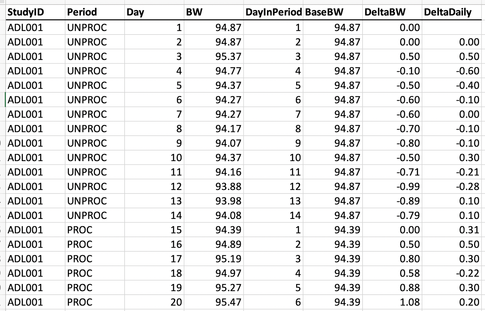
In this spreadsheet, each row tells us about the weight for one participant on one day of the 4-week-long study. These daily body weight measurements were performed at 6am each morning, so we have one row for every day.
Let’s also orient you to the columns. “StudyID” is the ID for each participant. Here we can see that in this screenshot we are looking just at participant ADL001, or participant 01 for short. The “Period” variable tells us whether the participant was eating an ultra-processed (PROC) or an unprocessed (UNPROC) diet on that day. Here we can see that participant 01 was part of the group who had an unprocessed diet for the first two weeks, before switching to the ultra-processed diet for the last two weeks. “Day” tells us which day in the 28-day study the measurement is from. Here we show only the first 20 days for participant 01.
“BW” is the main variable of interest, as it is the participant’s measured weight, in kilograms, for that day of the study. “DayInPeriod” tells us which day they are on for that particular diet. Each participant goes 14 days on one diet then begins day 1 on the other diet. “BaseBW” is just their weight for day 1 on that period. Participant 01 was 94.87 kg on day one of the unprocessed diet, so this column holds that value as long as they’re on that diet. “DeltaBW” is the difference between their weight on that day and the weight they were at the beginning of that period. For example, participant 01 weighed 94.87 kg on day one and 94.07 kg on day nine, so the DeltaBW value for day nine is -0.80.
Finally, “DeltaDaily” is a variable that we added, which is just a simple calculation of how much the participant’s weight changed each day. If someone weighed 82.85 kg yesterday and they weigh 82.95 kg today, the DeltaDaily would be 0.10, because they gained 0.10 kg in the last 24 hours.
To begin with, we were able to replicate the authors’ main findings. When we don’t round to one decimal place, we see that participants on the ultra-processed diet gained an average of 0.9380 (± 0.3219) kg, and participants on the unprocessed diet lost an average of 0.9085 (± 0.3006) kg. That’s only a difference of 0.0295 kg in absolute values in the means, and 0.0213 kg for the standard errors, which we still find quite surprising. Note that this is different from the concern about standard errors raised by Drs. Mackerras and Blizzard. Many of the standard errors in this paper come from GLM analysis, which assumes homogeneity of variances and often leads to identical standard errors. But these are independently calculated standard errors of the mean for each condition, so it is still somewhat surprising that they are so similar (though not identical).
On average these participants gained and lost impressive, but not shocking amounts of weight. A few of the participants, however, saw weight loss that was very concerning. One woman lost 4.3 kg in 14 days which, to quote Nick Brown, “is what I would expect if she had dysentery” (evocative though perhaps a little excessive). In fact, according to the data, she lost 2.39 kg in the first five days alone. We also notice that this patient was only 67.12 kg (about 148 lbs) to begin with, so such a huge loss is proportionally even more concerning. This is the most extreme case, of course, but not the only case of such intense weight change over such a short period.
The article tells us that participants were weighed on a Welch Allyn Scale-Tronix 5702 scale, which has a resolution of 0.1 lb or 100 grams (0.1 kg). This means it should only display data to one decimal place. Here’s the manufacturer’s specification sheet for that model. But participant weights in the file deltabw are all reported to two decimal places; that is, with a precision of 0.01 kg, as you can clearly see from the screenshot above. Of the 560 weight readings in the data file, only 55 end in zero. It is not clear how this is possible, since the scale apparently doesn’t display this much precision.

To confirm this, we wrote to Welch Allyn’s customer support department, who confirmed that the model 5702 has 0.1 kg resolution.
We also considered the possibility that the researchers measured people’s weight in pounds and then converted to kilograms, in order to use the scale’s better precision of 0.1 pounds (45.4 grams) rather than 100 grams. However, in this case, one would expect to see that all of the changes in weight were multiples of (approximately) 0.045 kg, which is not what we observe.
III.
As we look closer at the numbers, things get even more confusing.
As we noted, Hall et al. report participant weight to two decimal places in kilograms for every participant on every day. Kilograms to two decimal places should be pretty sensitive, but there are many cases where the exact same weight appears two or even three times in a row. For example, participant 21 is listed as having a weight of exactly 59.32 kg on days 12, 13, and 14, participant 13 is listed as having a weight of exactly 96.43 kg on days 10, 11, and 12, and participant 06 is listed as having a weight of exactly 49.54 kg on days 23, 24, and 25.
Having the same weight for two or even three days in a row may not seem that strange, but it is very remarkable when the measurement is in kilograms precise to two decimal places. After all, 0.01 kg (10 grams) is not very much weight at all. A standard egg weighs about 0.05 kg (50 grams). A shot of liquor is a little less, usually a bit more than 0.03 kg (30 grams). A tablespoon of water is about 0.015 kg (15 grams). This suggests that people’s weights are varying by less than the weight of a tablespoon of water over the course of entire days, and sometimes over multiple days. This uncanny precision seems even more unusual when we note that body weight measurements were taken at 6 am every morning “after the first void”, which suggests that participants’ bodily functions were precise to 0.01 kg on certain days as well.
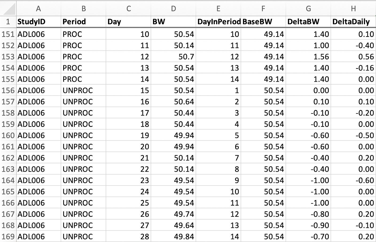
The case of participant 06 is particularly confusing, as 49.54 kg is exactly one kilogram less, to two decimal places, than the baseline for this participant’s weight when they started, 50.54 kg. Furthermore, in the “unprocessed” period, participant 06 only ever seems to lose or gain weight in full increments of 0.10 kilograms.
We see similar patterns in the data from other participants. Let’s take a look at the DeltaDaily variable. As a reminder, this variable is just the difference between a person’s weight on one day and the day before. These are nothing more than daily changes in weight.
Because these numbers are calculated from the difference between two weight measurements, both of which are reported to two decimal places of accuracy, these numbers should have two places of accuracy as well. But surprisingly, we see that many of these weight changes are in full increments of 0.10.
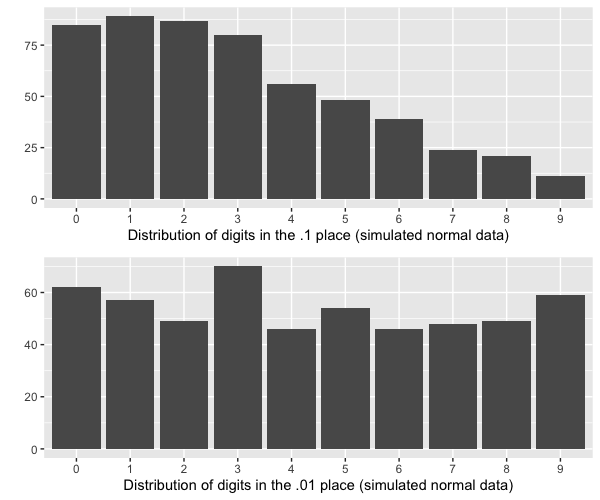
Take a look at the histograms below. The top histogram is the distribution of weight changes by day. For example, a person might gain 0.10 kg between days 15 and 16, and that would be one of the observations in this histogram.
You’ll see that these data have an extremely unnatural hair-comb pattern of spikes, with only a few observations in between. This is because the vast majority (~71%) of the weight changes are in exact multiples of 0.10, despite the fact that weights and weight changes are reported to two decimal places. That is to say, participants’ weights usually changed in increments like 0.20 kg, -0.10 kg, or 0.40 kg, and almost never in increments like -0.03 kg, 0.12 kg, or 0.28 kg.
For comparison, on the bottom is a sample from a simulated normal distribution with identical n, mean, and standard deviation. You’ll see that there is no hair-comb pattern for these data.
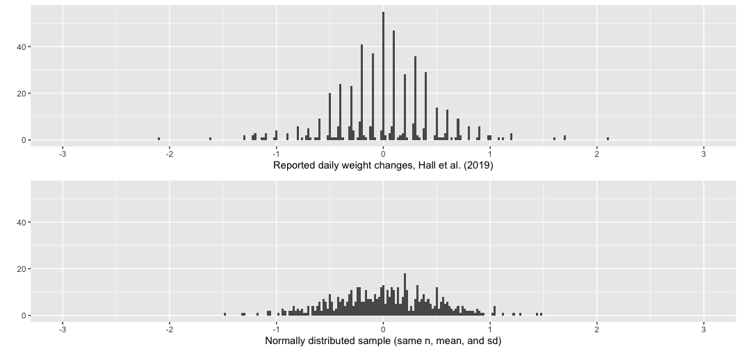
As we mentioned earlier, there are several cases where a participant stays at the exact same weight for two or three days in a row. The distribution we see here is the cause. As you can see, the most common daily change is exactly zero. Now, it’s certainly possible to imagine why some values might end up being zero in a study like this. There might be a technical incident with the scale, a clerical error, or a mistake when recording handwritten data on the computer. A lazy lab assistant might lose their notes, resulting in the previous day’s value being used as the reasonable best estimate. But since a change of exactly zero is the modal response, a full 9% of all measurements, it’s hard to imagine that these are all omissions or technical errors.
In addition, there’s something very strange going on with the trailing digits:
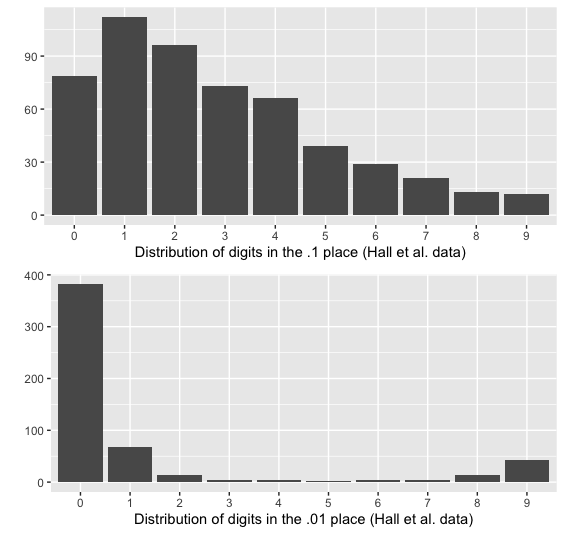
On the top here we have the distribution of digits in the 0.1 place. For example, a measurement of 0.29 kg would appear as a 2 here. This follows about the distribution we would expect, though there are a few more 1’s and fewer 0’s than usual.
The bottom histogram is where things get weird. Here we have the distribution of digits in the 0.01 place. For example, a measurement of 0.29 kg would appear as a 9 here. As you can see, 382/540 of these observations have a 0 in their 0.01’s place — this is the same as that figure of 71% of measured changes being in full increments of 0.10 kg that we mentioned earlier.
The rest of the distribution is also very strange. When the trailing digit is not a zero, it is almost certainly a 1 or a 9, possibly a 2 or an 8, and almost never anything else. Of 540 observed weight changes, only 3 have a trailing digit of 5.
We can see that this is not what we would expect from (simulated) normally distributed data:
It’s also not what we would expect to see if they were measuring to one decimal place most of the time (~70%), but to two decimal places on occasion (~30%). As we’ve already mentioned, this doesn’t make sense from a methodological standpoint, because all daily weights are to two decimal places. But even it somehow were a measurement accuracy issue, we would expect an equal distribution across all the other digits besides zero, like this:

This is certainly not what we see in the reported data. The fact that 1 and 9 are the most likely trailing digit after 0, and that 2 and 8 are most likely after that, is especially strange.
IV.
When we first started looking into this paper, we approached Retraction Watch, who said they considered it a potential story. After completing the analyses above, we shared an early version of this post with Retraction Watch, and with our permission they approached the authors for comment. The authors were kind enough to offer feedback on what we had found, and when we examined their explanation, we found that it clarified a number of our points of confusion.
The first thing they shared with us was this erratum from October 2020, which we hadn’t seen before. The erratum reports that they noticed an error in the documented diet order of one participant. This is an important note but doesn’t affect the analyses we present here, which have very little to do with diet conditions.
Kevin Hall, the first author on this paper, also shared a clarification on how body weights were calculated:
I think I just discovered the likely explanation about the distribution of high-precision digits in the body weight measurements that are the main subject of one of the blogs. It’s kind of illustrative of how difficult it is to fully report experimental methods! It turns out that the body weight measurements were recorded to the 0.1 kg according to the scale precision. However, we subtracted the weight of the subject’s pajamas that were measured using a more precise balance at a single time point. We repeated subtracting the mass of the pajamas on all occasions when the subject wore those pajamas. See the example excerpted below from the original form from one subject who wore the same pajamas (PJs) for three days and then switched to a new set. Obviously, the repeating high precision digits are due to the constant PJs! 😉
This matches what is reported in the paper, where they state, “Subjects wore hospital-issued top and bottom pajamas which were pre-weighed and deducted from scale weight.”
Kevin also included the following image, which shows part of how the data was recorded for one participant:
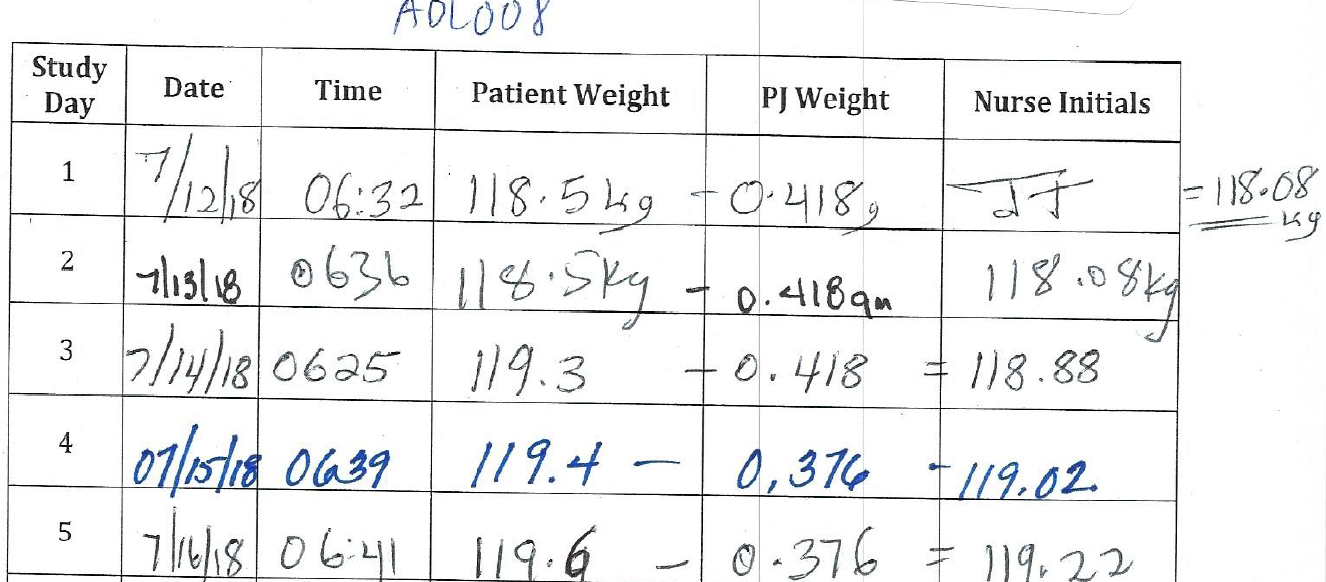
If we understand this correctly, the first time a participant wore a set of pajamas, the pajamas were weighed to three decimals of precision. Then, that measurement was subtracted from the participant’s weight on the scale (“Patient Weight”) on every consecutive morning, to calculate the participant’s body weight. For an unclear reason, this was recorded to two decimals of precision, rather than the one decimal of precision given by the scale, or the three decimals of precision given by the PJ weights. When the participant switched to a new set of pajamas, the new set was weighed to three decimals of precision, and that number was used to calculate participant body weight until they switched to yet another new set of pajamas, etc.
We assume that the measurement for the pajamas is given in kilograms, even though they write “g” and “gm” (“qm”?) in the column. I wish my undergraduate lab TAs were as forgiving as the editors at Cell Metabolism.
This method does account for the fact that participant body weights were reported to two decimal places of precision, despite the fact that the scale only measures weight to one decimal place of precision. Even so, there were a couple of things that we still found confusing.
The variable that interests us the most is the DeltaDaily variable. We can easily calculate that variable for the provided example, like so:
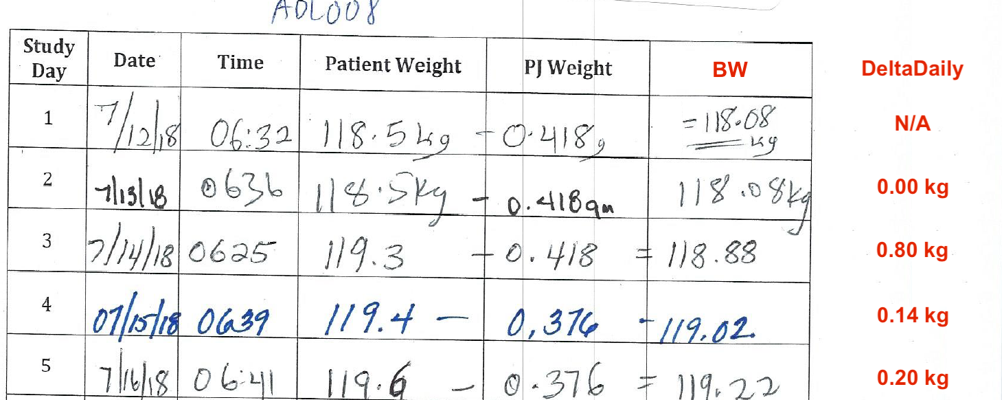
We can see that whenever a participant doesn’t change their pajamas on consecutive days, there’s a trailing zero. In this way, the pajamas can account for the fact that 71% of the time, the trailing digits in the DeltaDaily variable were zeros.
We also see that whenever the trailing digit is not zero, that lets us identify when a participant has changed their pajamas. Note of course that about ten percent of the time, a change in pajamas will also lead to a trailing digit of zero. So every trailing digit that isn’t zero is a pajama change, though a small number of the zeros will also be “hidden” pajama changes.
In any case, we can use this to make inferences about how often participants change their pajamas, which we find rather confusing. Participants often change their pajamas every day for multiple days in a row, or go long stretches without apparently changing their pajamas at all, and sometimes these are the same participants. It’s possible that these long stretches without any apparent change of pajamas are the result of the “hidden” changes we mentioned, because about 10% of the time changes would happen without the trailing digit changing, but it’s still surprising.
For example, participant 05 changes their pajamas on day 2, day 5, and day 10, and then apparently doesn’t change their pajamas again until day 28, going more than two weeks without a change in PJs. Participant 20, in contrast, changes pajamas at least 16 times over 28 days, including every day for the last four days of the study. The record for this, however, has to go to participant 03, who at one point appears to have switched pajamas every day for at least seven days in a row. Participant 03 then goes eight days in a row without changing pajamas before switching pajamas every day for three days in a row.
Participant 08 (the participant from the image above) seems to change their pajamas only twice during the entire 28-day study, once on day 4 and again on day 28. Certainly this is possible, but it doesn’t look like the pajama-wearing habits we would expect. It’s true that some people probably want to change their pajamas more than others, but this doesn’t seem like it can be entirely attributed to personality, as some people don’t change pajamas at all for a long time, and then start to change them nearly every day, or vice-versa.
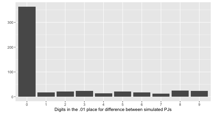
We were also unclear on whether the pajamas adjustment could account for the most confusing pattern we saw in the data for this article, the distribution of digits in the .01 place for the DeltaDaily variable:
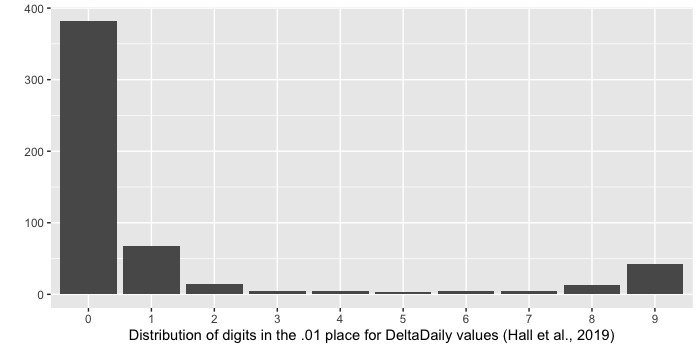
The pajamas method can explain why there are so many zeros — any day a participant didn’t change their pajamas, there would be a zero, and it’s conceivable that participants only changed their pajamas on 30% of the days they were in the study.
We weren’t sure if the pajamas method could explain the distribution of the other digits. For the trailing digits that aren’t zero, 42% of them are 1’s, 27% of them are 9’s, 9% of them are 2’s, 8% of them are 8’s, and the remaining digits account for only about 3% each. This seems very strange.
You’ll recall that the DeltaDaily values record the changes in participant weights between consecutive days. Because the weight of the scale is only precise to 0.1 kg, the data in the 0.01 place records information about the difference between two different pairs of pajamas. For illustration, in the example Kevin Hall provided, the participant switched between a pair of pajamas weighing 0.418 kg and a pair weighing 0.376 kg. These are different by 0.042 kg, so when they rounded it to two digits, the difference we see in the DeltaDaily has a trailing digit of 4.
We wanted to know if the pajama adjustment could explain why the difference (for the digit in the 0.01’s place) between the weights of two pairs of pajamas are 14x more likely to be a 1 than a 6, or 9x more likely to be a 9 than a 3.
Verbal arguments quickly got very confusing, so we decided to run some simulations. We simulated 20 participants, for 28 days each, just like the actual study. On day one, simulated participants were assigned a starting weight, which was a random integer between 40 and 100. Every day, their weight changed by an amount between -1.5 and 1.5 by increments of 0.1 (-1.5, -1.4, -1.3 … 1.4, 1.5), with each increment having an equal chance of occuring.
The important part of the simulation were the pajamas, of course. Participants were assigned a pajama weight on day 1, and each day they had a 35% chance of changing pajamas, and being assigned a new pajama weight. The real question was how to generate a reasonable distribution of pajama weights. We didn’t have much to go off of, just the two values in the image that Kevin Hall shared with us. But we decided to give it a shot with just that information. Weights of 418 g and 376 g have a mean of just under 400 g and a standard deviation of 30 g, so we decided to sample our pajama weights from a normal distribution with those parameters.
When we ran this simulation, we found a distribution of digits in the 0.01 place that didn’t show the same saddle-shaped distribution as in the data from the paper:
We decided to run some additional simulations, just to be sure. To our surprise, when the SD of the pajamas is smaller, in the range of 10-20 g, you can sometimes get saddle-shaped distributions just like the ones we saw in data from the paper. Here’s an example of what the digits can look like when the SD of the pajamas is 15 g:
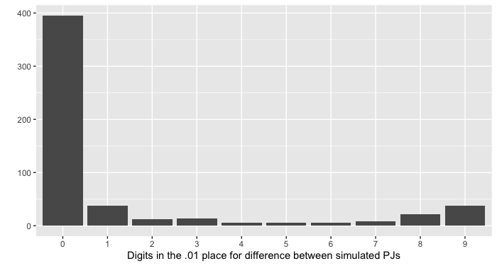
It’s hard for us to say whether a standard deviation of 15 g or of 30 g is more realistic for hospital pajamas, but it’s clear that under certain circumstances, pajama adjustments can create this kind of distribution (we propose calling it the “pajama distribution”).
While we find this distribution surprising, we conclude that it is possible given what we know about these data and how the weights were calculated.
V.
When we took a close look at these data, we originally found a number of patterns that we were unable to explain. Having communicated with the authors, we now think that while there are some strange choices in their analysis, most of these patterns can be explained when we take into account the fact that pajama weights were deducted from scale weights, and the two weights had different levels of precision.
While these patterns can be explained by the pajama adjustment described by Kevin Hall, there are some important lessons here. The first, as Kevin notes in his comment, is that it can be very difficult to fully record one’s methods. It would have been better to include the full history of this variable in the data files, including the pajama weights, instead of recording the weights and performing the relevant comparisons by hand.
The second is a lesson about combining data of different levels of precision. The hair-comb pattern that we observed in the distribution of DeltaDaily scores was truly bizarre, and was reason for serious concern. It turns out that this kind of distribution can occur when a measure with one decimal of precision is combined with another measure with three decimals of precision, with the result being rounded to two decimals of precision. In the future researchers should try to avoid combining data in this way to avoid creating such artifacts. While it may not affect their conclusions, it is strange for the authors to claim that someone’s weight changed by (for example) 1.27 kg, when they have no way to measure the change to that level of precision.
There are some more minor points that this explanation does not address, however. We still find it surprising how consistent the weight change was in this study, and how extreme some of the weight changes were. We also remain somewhat confused by how often participants changed (or didn’t change) their pajamas.
This post continues in Part Two over at Nick Brown’s blog, where he covers several other aspects of the study design and data.
Thanks again to Nick Brown for comparing notes with us on this analysis, to James Heathers for helpful comments, and to a couple of early readers who asked to remain anonymous. Special thanks to Kevin Hall and the other authors of the original paper, who have been extremely forthcoming and polite in their correspondence. We look forward to ongoing public discussion of these analyses, as we believe the open exchange of ideas can benefit the scientific community.

This pajama stuff seems like an example of the perfect being the enemy of the good. Since the delta in the weights of different pajamas was less than the precision of the scale, there really was no need to do these elaborate pajama calculations, but it _feels_ like you’re improving your experiment by eliminating a tiny source of error.
I wish there was a slightly more informative version of https://xkcd.com/2295/ to be hung on the wall of every medical/psych/stats-using discipline
LikeLiked by 1 person
This is a really good point! The pajamas appear to have been always within a couple dozen grams of 400 g, so there’s almost no noise to account for in the first place. Thanks for mentioning this!
LikeLike
You guys are just amamzing. But why could they not weigh the subjects in the nude?
LikeLike
Ethical reasons I expect.
LikeLike
Wait a minute. According to that paper, salted roast peanuts are “ultra-processed”? The nutritionists are on their bullshit again.
LikeLike