Peer Review: Obesity II – Establishing Causal Links Between Chemical Exposures and Obesity

A new paper, called Obesity II: Establishing Causal Links Between Chemical Exposures and Obesity, was just published in the journal Biochemical Pharmacology (available online as of 5 April 2022). Authors include some obesity bigwigs like Robert H. Lustig, and it’s really long, so we figured it might be important. 

The title isn’t some weird Walden II reference — there’s a Part I and Part III as well. Part I reviews the obesity epidemic (in case you’re not already familiar?) and argues that obesity “likely has origins in utero.”

“The obesity epidemic is Kurt Cobain’s fault” is an unexpected but refreshing hypothesis

Part III basically argues that we should move away from doing obesity research with cells isolated in test tubes (probably a good idea TBH) and move towards “model organisms such as Drosophila, C. elegans, zebrafish, and medaka.” Sounds fishy to us but whatever, you’re the doctor.

This paper, Part II, makes the case that environmental contaminants “play a vital role in” the obesity epidemic, and presents the evidence in favor of a long list of candidate contaminants. We’re going to stick with Part II today because that’s what we’re really interested in.

For some reason the editors of this journal have hidden away the peer reviews instead of publishing them alongside the paper, like any reasonable person would. After all, who could possibly evaluate a piece of research without knowing what three anonymous faculty members said about it? The editors must have just forgotten to add them. But that’s ok — WE are these people’s peers as well, so we would be happy to fill the gap. Consider this our peer review:

This is an ok paper. They cite some good references. And they do cite a lot of references (740 to be exact), which definitely took some poor grad students a long time and should probably count for something. But the only way to express how we really feel is:

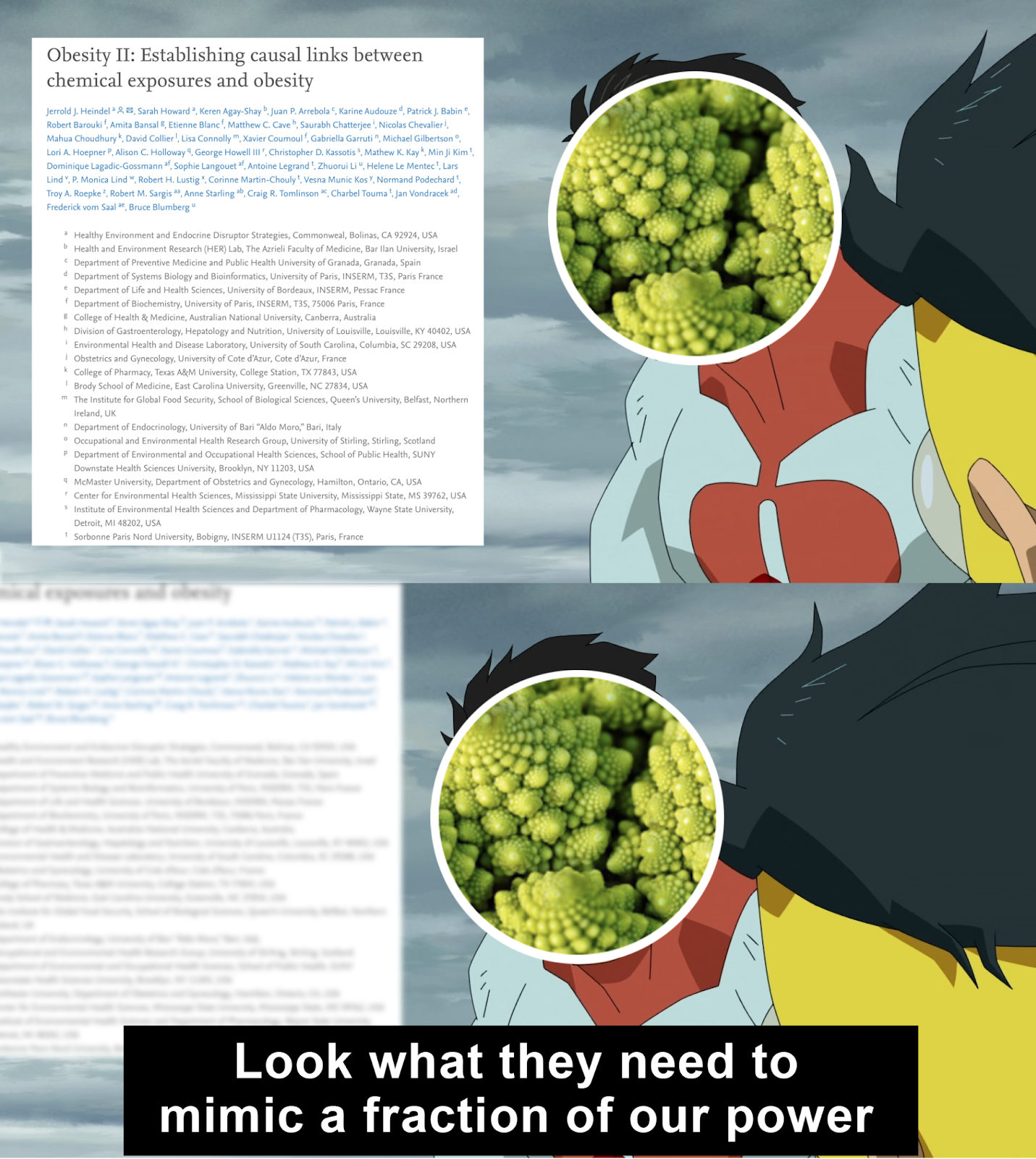
Seriously, 43 authors from 33 different institutions coming together to tell you that “ubiquitous environmental chemicals called obesogens play a vital role in the obesity pandemic”? We could have told you that a year ago, on a budget of $0. 

This wasted months, maybe years of their lives, and millions of taxpayer dollars making this paper that is just like, really boring and not very good. Meanwhile we wrote the first draft of A Chemical Hunger in a month (pretty much straight through in October 2020) and the only reason you didn’t see it sooner was because we were sending drafts around to specialists to make sure there wasn’t anything major that we overlooked (there wasn’t).

We don’t want to pick on the actual authors because, frankly, we’re sure this paper must have been a nightmare to work on. Most of the authors are passengers of this trainwreck — involved, but not responsible. We blame the system they work under.

We hope this doesn’t seem like a priority dispute. We don’t claim priority for the contamination hypothesis — here are four papers from 2008, 2009, 2010, and 2014, way before our work on the subject, all arguing in favor of the idea that contaminants cause obesity. If the contamination hypothesis turns out to be right, give David B. Allison the credit, or maybe someone even earlier. We just think we did an exceptionally good job making the case for the hypothesis. Our only original contributions (so far) are arguing that the obesity epidemic is 100% (ok, >90%) caused by contaminants, and suggesting lithium as a likely candidate. 

So we’re not trying to say that these authors are a bunch of johnny-come-latelies (though they kind of are, you see the papers up there from e.g. 2008?). The authors are victims here of a vicious system that has put them in such a bad spot that, for all their gifts, they can now only produce rubbish papers, and we think they know this in their hearts. It’s no wonder grad students are so depressed! 

So to us, this paper looks like a serious condemnation of the current academic system, and of the medical research system in particular. And while we don’t want to criticize the researchers, we do want to criticize the paper for being an indecisive snoozefest.

Long Paper is Long

The best part of this paper is that comes out so strongly against “traditional wisdom” about the obesity epidemic:  

The prevailing view is that obesity results from an imbalance between energy intake and expenditure caused by overeating and insufficient exercise. We describe another environmental element that can alter the balance between energy intake and energy expenditure: obesogens. … Obesogens can determine how much food is needed to maintain homeostasis and thereby increase the susceptibility to obesity. 

In particular we like how they point out how, from the contaminant perspective, measures of how much people eat are just not that interesting. If chemicals in your carpet raise your set point, you may need to eat more just to maintain homeostasis, and you might get fat. This means that more consumption, of calories or anything else you want to measure, is consistent with contaminants causing obesity. We made the same point in Interlude A. Anyways, don’t come at us about CICO unless you’ve done your homework. 

We also think the paper’s heart is in the right place in terms of treatment: 

The focus in the obesity field has been to reduce obesity via medicines, surgery, or diets. These interventions have not been efficacious as most people fail to lose weight, and even those who successfully lose substantial amounts of weight regain it. A better approach would be to prevent obesity from occurring in the first place. … A significant advantage of the obesogen hypothesis is that obesity results from an endocrine disorder and is thus amenable to a focus on prevention. 

So for this we say: preach, brothers and sisters.

The rest of the paper is boring to read and inconclusive. If you think we’re being unfair about how boring it is, we encourage you to go try to read it yourself.

Specific Contaminants

The paper doesn’t even do a good job assessing the evidence for the contaminants it lists. For example, glyphosate. Here is their entire review:

Glyphosate is the most used herbicide globally, focusing on corn, soy and canola [649]. Glyphosate was negative in 3T3-L1 adipogenic assays [650], [651]. Interestingly, three different formulations of commercial glyphosate, in addition to glyphosate itself, inhibited adipocyte proliferation and differentiation from 3T3-L1 cells [651]. There are also no animal studies focusing on developmental exposure and weight gain in the offspring. An intriguing study exposed pregnant rats to 25mg/kg/day during days 8-14 of gestation [652]. The offspring were then bred within the lineage to generate F2 offspring and bread to generate the F3 progeny. About 40% of the males and females of the F2 and F3 had abdominal obesity and increased adipocyte size revealing transgenerational inheritance. Interestingly, the F1 offspring did not show these effects. These results need verification before glyphosate can be designated as an obesogen.

For comparison, here’s our review of glyphosate. We try to, you know, come to a conclusion. We spend more than a paragraph on it. We cite more than four sources.

We cite their [652] as well, but we like, ya know, evaluate it critically and in the context of other exposure to the same compound. We take a close look at our sources, and we tell the reader we don’t think glyphosate is a major contributor to the obesity epidemic because the evidence doesn’t look very strong to us. This is bare-bones due diligence stuff. Take a look: 

The best evidence for glyphosate causing weight gain that we could find was from a 2019 study in rats. In this study, they exposed female rats (the original generation, F0) to 25 mg/kg body weight glyphosate daily, during days 8 to 14 of gestation. There was essentially no effect of glyphosate exposure on these rats, or in their children (F1), but there was a significant increase in the rates of obesity in their grandchildren (F2) and great-grandchildren (F3). There are some multiple comparison issues, but the differences are relatively robust, and are present in both male and female descendants, so we’re inclined to think that there’s something here. 

There are a few problems with extending these results to humans, however, and we don’t just mean that the study subjects are all rats. The dose they give is pretty high, 25 mg/kg/day, in comparison to (again) farmers working directly with the stuff getting a dose closer to 0.004 mg/kg.

The timeline also doesn’t seem to line up. If we take this finding and apply it to humans at face value, glyphosate would only make you obese if your grandmother or great-grandmother was exposed during gestation. But glyphosate wasn’t brought to market until 1974 and didn’t see much use until the 1990s. There are some grandparents today who could have been exposed when they were pregnant, but obesity began rising in the 1980s. If glyphosate had been invented in the 1920s, this would be much more concerning, but it wasn’t.

Frankly, if they aren’t going to put in the work to engage with studies at this level, they shouldn’t have put them in this review. 

If this were a team of three people or something, that would be one thing. But this is 43 specialists working on this problem for what we assume was several months. We wrote our glyphosate post in maybe a week?

Some of the reviews are better than this — their review of BPA goes into more detail and cites a lot more studies. But the average review is pretty cruddy. For example, here’s the whole review for MSG:

Monosodium glutamate (MSG) is a flavor enhancer used worldwide. Multiple animal studies provided causal and mechanistic evidence that parenteral MSG intake caused increased abdominal fat, dyslipidemia, total body weight gain, hyperphagia and T2D by affecting the hypothalamic feeding center [622], [623], [624]. MSG increased glucagon-like peptide-1 (GLP-1) secretion from the pGIP/neo: STC-1 cell line indicating a possible action on the gastrointestinal (GI) tract in addition to its effects on the brain [625]. It is challenging to show similar results in humans because there is no control population due to the ubiquitous presence of MSG in foods. MSG is an obesogen.

Seems kind of extreme to unequivocally declare “MSG is an obesogen” on the basis of just four papers. On the basis of results that seem to be in mice, rats, mice, and cells in a test tube, as far as we can tell (two of the citations are review articles, which makes it hard for us to know what studies they specifically had in mind). Somehow this is enough to declare MSG a “Class I Obesogen” — Animal evidence: Strong. In vitro evidence: Strong. Regulatory action: to be banned. Really? 

Instead, we support the idea of — thinking about it for five minutes. For example, MSG occurs naturally in many foods. If MSG were a serious obesogen, tomatoes and dashi broth would both make you obese. Why are Italy and Japan not more obese? The Japanese first purified MSG and they love it so much, they have a factory tour for the stuff that is practically a theme park — “there is a 360-degree immersive movie experience, a diorama and museum of factory history, a peek inside the fermentation tanks (yum!), and finally, an opportunity to make and taste your own MSG seasoning.” Yet Japan is one of the leanest countries in the world.

As far as we can tell, Asia in general consumes way more MSG than any other part of the world. “Mainland China, Indonesia, Vietnam, Thailand, and Taiwan are the major producing countries in Asia.” Why are these countries not more obese? MSG first went on the market in 1909. Why didn’t the obesity epidemic start then? We just don’t think it adds up. 

(Also kind of weird to put this seasoning invented in Asia, and most popular in Asia, under your section on “Western diet.”)

Adapted from Fig. 3

Let’s also look at their section on DDT. This one, at least, is several paragraphs long, so we won’t quote it in full. But here’s the summary: 

A 2017 systematic review of in vitro, animal and epidemiological data on DDT exposures and obesity concluded the evidence indicated that DDT was “presumed” to be obesogenic for humans [461]. The in vitro and animal data strongly support DDT as an obesogen. Based on the number of positive prospective human studies, DDT is highly likely to be a human obesogen. Animal and human studies showed obesogenic transmission across generations. Thus, a POP banned almost 50 years ago is still playing a role in the current obesity pandemic, which indicates the need for caution with other chemical exposures that can cause multigenerational effects.

We’re open to being convinced otherwise, but again, this doesn’t really seem to add up. DDT was gradually banned across different countries and was eventually banned worldwide. Why do we not see reversals or lags in the growth of obesity in those countries those years? They mention that DDT is still used in India and Africa, sometimes in defiance of the ban. So why are obesity rates in India and Africa so low? We’d love to know what they think of this and see it contextualized more in terms of things like occupation and human exposure timeline.

Review Paper

With a long list of chemicals given only the briefest examination, it’s hard not to see this paper as overly inclusive to the point of being useless. It makes the paper feel like a cheap land grab to stake a claim to being correct in the future if any of the chemicals on the list pan out.

Maybe their goal is just to list and categorize every study that has ever been conducted that might be relevant. We can sort of understand this but — why no critical approach to the material? Which of these studies are ruined by obvious confounders? How many of them have been p-hacked to hell? Seems like the kind of thing you would want to know! 

You can’t just list papers and assume that it will get you closer to understanding. In medicine, the reference for this problem is Ioannidis’s Why Most Published Research Findings Are False. WMPRFAF was published in 2005, you don’t have an excuse for not thinking critically about your sources.

Despite this, they don’t even mention lithium, which seems like an oversight. 

Oh right, Kurt Cobain IS responsible for the obesity epidemic

We wish the paper tried to provide a useful conclusion. It would have been great to read them making their best case for pretty much anything. Contaminants are responsible for 50% of the epidemic. Contaminants are responsible for no more than 10% of the epidemic. Contaminants are responsible for more than 90% of the epidemic. We think phthalates are the biggest cause. We think DDT is the biggest cause. We think it’s air pollution and atrazine. Make a case for something. That would be cool.

What is not cool is showing up being like: Hey we have a big paper! The obesity epidemic is caused by chemicals, perhaps, in what might possibly be your food and water, or at work, though if it’s not, they aren’t. This is a huge deal if this is what caused the epidemic, possibly, unless it didn’t. The epidemic is caused by any of these several dozen compounds, unless it’s just one, or maybe none of them. What percentage of the epidemic is caused by these compounds? It’s impossible to say. But if we had to guess, somewhere between zero and one hundred percent. Unless it isn’t. 

Effect Size

The paper spends almost no time talking about effect size, which we think is 1) a weird choice and 2) the wrong approach for this question. 

We don’t just care about which contaminants make you gain weight. We care about which contaminants make you gain a concerning amount of weight. We want to know which contaminants have led to the ~40 lbs gain in average body weight since 1970, not which of them can cause 0.1 lbs of weight gain if you’re inhaling them every day at work. These differences are more than just important, they’re the question we’re actually interested in!

For comparison: coffee and airplane travel are both carcinogens, but they increase your risk of cancer by such a small degree that it’s not even worth thinking about, unless you’re a pilot with an espresso addiction. When the paper says “Chemical ABC is an obesogen”, it would be great to see some analysis of whether it’s an obesogen like how getting 10 minutes of sunshine is a carcinogen, or whether it’s an obesogen like how spending a day at the Chernobyl plant is a carcinogen. Otherwise we’re on to “bananas are radioactive” levels of science reporting — technically true, but useless and kind of misleading.

The huge number of contaminants they list does seem like a mark in favor of a “the obesity epidemic is massively multi-causal” hypothesis (which we discussed a bit in this interview), but again it’s hard to tell without seeing a better attempt to estimate effect sizes. The closest thing to an estimate that we saw was this line: “Population attributable risk of obesity from maternal smoking was estimated at 5.5% in the US and up to 10% in areas with higher smoking rates”.

Stress Testing

Their conclusion is especially lacking. It’s one thing to point out that what we’re studying is hard, but it’s another thing to deny the possibility of victory. Let’s look at a few quotes:

“A persistent key question is what percent of obesity is due to genetics, stress, overnutrition, lack of exercise, viruses, drugs or obesogens? It is virtually impossible to answer that question for any contributing factors… it is difficult to determine the exact effects of obesogens on obesity because each chemical is different, people are different, and exposures vary regionally and globally.”

Imagine going to an oncology conference and the keynote speaker gets up and says, “it is difficult to determine the exact effects of radiation on cancer because each radiation source is different, people are different, and exposures vary regionally and globally”. While much of this is true, oncologists don’t say this sort of thing (we hope?) because they understand that while the problem is indeed hard, it’s important, and hold out hope that solving that problem is not “virtually impossible”. Indeed, we’re pretty sure it’s not. 

They’re pretty pessimistic about future research options:

“We cannot run actual ‘clinical trials’ where exposure to obesogens and their effects are monitored over time. Thus, we focus on assessing the strength of the data for each obesogen.”

Assessing the strength of the data is a good idea, but this is leaving a lot on the table. Natural experiments are happening all the time, and you don’t need clinical trials to infer causality. We’d like to chastise this paper with the following words:

[Before] we set about instructing our colleagues in other fields, it will be proper to consider a problem fundamental to our own. How in the first place do we detect these relationships between sickness, injury and conditions of work? How do we determine what are physical, chemical and psychological hazards of occupation, and in particular those that are rare and not easily recognized?

There are, of course, instances in which we can reasonably answer these questions from the general body of medical knowledge. A particular, and perhaps extreme, physical environment cannot fail to be harmful; a particular chemical is known to be toxic to man and therefore suspect on the factory floor. Sometimes, alternatively, we may be able to consider what might a particular environment do to man, and then see whether such consequences are indeed to be found. But more often than not we have no such guidance, no such means of proceeding; more often than not we are dependent upon our observation and enumeration of defined events for which we then seek antecedents.

… However, before deducing ‘causation’ and taking action we shall not invariably have to sit around awaiting the results of the research. The whole chain may have to be unraveled or a few links may suffice. It will depend upon circumstances.

Sir Austin Bradford Hill said that, and we’d say he knows a little more about clinical trials than you do, pal, because HE INVENTED THEM. And then he perfected them so that no living physician could best him in the Ring of Honor– 

So we think the “no clinical trials” thing is a non-issue. Sir Austin Bradford Hill and colleagues were able to discover the connection between cigarette smoking and lung cancer without forcing people to smoke more than they were already smoking. You really can do medical research without clinical trials.

They did not do this

But even so, the paper is just wrong. We can run clinical trials. People do occasionally lose weight, sometimes huge amounts of weight. So we can try removing potential obesogens from the environment and seeing if that leads to weight loss. If we do it in a controlled manner, we can get some pretty strong evidence about whether or not specific contaminants are causing obesity.

Defeatism

Our final and biggest problem with this paper is that it is so tragically defeatist. It leaves you totally unsure as to what would be informative additional research. It doesn’t show a clear path forward. It’s pessimistic. And it’s tedious as hell. All of this is bad for morale. 

The paper’s suggestions seem like a list of good ways to spend forever on this problem and win as many grants as possible. This seems “good” for the scientists in the narrow sense that it will help them keep their tedious desk jobs, jobs which we think they all secretly hate. It’s “good” in that it lets you keep playing what Erik Hoel describes as “the Science Game” for as long as possible:

When you have a lab, you need grant money. Not just for yourself, but for the postdoctoral researchers and PhDs who depend on you for their livelihoods. … much of what goes on in academia is really the Science Game™. … varying some variable with infinite degrees of freedom and then throwing statistics at it until you get that reportable p-value and write up a narrative short story around it.

Think of it like grasping a dial, and each time you turn it slightly you produce a unique scientific publication. Such repeatable mechanisms for scientific papers are the dials everyone wants. Playing the Science Game™ means asking a question with a slightly different methodology each time, maybe throwing in a slightly different statistical analysis. When you’re done with all those variations, just go back and vary the original question a little bit. Publications galore.

If this is your MO, then “more research is needed” is the happiest sound in the world. Actually solving a problem, on the other hand, is kind of terrifying. You would need to find a new thing to investigate! It’s much safer to do inconclusive work on the same problem for decades.

This is part of why we find the suggestion to move towards research with “model organisms such as Drosophila, C. elegans, zebrafish, and medaka” so suspicious. Will this solve the obesity epidemic? Probably not, and certainly not any time this decade. Will it allow you to generate a lot of different papers on exposing Drosophila, C. elegans, zebrafish, and medaka to slightly different amounts of every chemical imaginable? Absolutely.

(As Paul Graham describes, “research must be substantial– and awkward systems yield meatier papers, because you can write about the obstacles you have to overcome in order to get things done. Nothing yields meaty problems like starting with the wrong assumptions.’”)

With all due respect to this approach, we do NOT want to work on obesity for the rest of our lives. We want to solve obesity in the next few years and move on to something else. We think that this is what you want to happen too! Wouldn’t it be nice to at least consider that we might make immediate progress on serious problems? What ever happened to that? 

Political Scientist Adolph Reed Jr. once wrote that modern liberalism has no particular place it wants to go. “Its métier,” he said, “is bearing witness, demonstrating solidarity, and the event or the gesture. Its reflex is to ‘send messages’ to those in power, to make statements, and to stand with or for the oppressed. This dilettantish politics is partly the heritage of a generation of defeat and marginalization, of decades without any possibility of challenging power or influencing policy.“

In this paper, we encounter a scientific tradition that no longer has any place it wants to go (“curing obesity? what’s that?”), that makes stands but has a hard time imagining taking action, that is the heir to a generation of defeat and marginalization. All that remains is a reflex of bearing witness to suffering. 

We think research can be better than this. That it can be active and optimistic. That it can dare to dream. That it can make an effort to be interesting. 

Why do we keep complaining about this paper being boring? Why does it matter? It matters because when the paper is boring, it suggests that the idea that obesity is caused by contaminants isn’t important enough to bother spending time on the writing. It suggests people won’t be interested to read the paper, that no one cares, that no care should be taken in the discussion. That nothing can be gained by thinking clearly about these ideas. It suggests that the prospect of curing obesity isn’t exciting. But we think that the prospect of curing obesity is very exciting, and we hope you do too!

A Chemical Hunger – Interlude B: The Nutrient Sludge Diet

[PART I – MYSTERIES]
[PART II – CURRENT THEORIES OF OBESITY ARE INADEQUATE]
[PART III – ENVIRONMENTAL CONTAMINANTS]
[INTERLUDE A – CICO KILLER, QU’EST-CE QUE C’EST?]
[PART IV – CRITERIA]
[PART V – LIVESTOCK ANTIBIOTICS]

In his book The Hungry Brain, neuroscientist Stephan Guyenet references a 1965 study in which volunteers received all their food from a “feeding machine” that pumped a “liquid formula diet” through a “dispensing syringe-type pump which delivers a predetermined volume of formula through the mouthpiece.” He devotes about three pages to the study, describing it like so:

What happens to food intake and adiposity when researchers dramatically restrict food reward? In 1965, the Annals of the New York Academy of Sciences published a very unusual study that unintentionally addressed this question. …

The “system” in question was a machine that dispensed liquid food through a straw at the press of a button—7.4 milliliters per press, to be exact (see figure 15). Volunteers were given access to the machine and allowed to consume as much of the liquid diet as they wanted, but no other food. Since they were in a hospital setting, the researchers could be confident that the volunteers ate nothing else. The liquid food supplied adequate levels of all nutrients, yet it was bland, completely lacking in variety, and almost totally devoid of all normal food cues.

The researchers first fed two lean people using the machine—one for sixteen days and the other for nine. Without requiring any guidance, both lean volunteers consumed their typical calorie intake and maintained a stable weight during this period.

Next, the researchers did the same experiment with two “grossly obese” volunteers weighing approximately four hundred pounds. Again, they were asked to “obtain food from the machine whenever hungry.” Over the course of the first eighteen days, the first (male) volunteer consumed a meager 275 calories per day—less than 10 percent of his usual calorie intake. The second (female) volunteer consumed a ridiculously low 144 calories per day over the course of twelve days, losing twenty-three pounds. The investigators remarked that an additional three volunteers with obesity “showed a similar inhibition of calorie intake when fed by machine.”

The first volunteer continued eating bland food from the machine for a total of seventy days, losing approximately seventy pounds. After that, he was sent home with the formula and instructed to drink 400 calories of it per day, which he did for an additional 185 days, after which he had lost two hundred pounds —precisely half his body weight. The researchers remarked that “during all this time weight was steadily lost and the patient never complained of hunger.” This is truly a starvation-level calorie intake, and to eat it continuously for 255 days without hunger suggests that something rather interesting was happening in this man’s body. Further studies from the same group and others supported the idea that a bland liquid diet leads people to eat fewer calories and lose excess fat.

This machine-feeding regimen was just about as close as one can get to a diet with zero reward value and zero variety. Although the food contained sugar, fat, and protein, it contained little odor or texture with which to associate them. In people with obesity, this diet caused an impressive spontaneous reduction of calorie intake and rapid fat loss, without hunger. Yet, strangely, lean people maintained weight on this regimen rather than becoming underweight. This suggests that people with obesity may be more sensitive to the impact of food reward on calorie intake.

In his review of the Hungry Brain, Scott Alexander provided a more concise description of the same study: 

In 1965, some scientists locked people in a room where they could only eat nutrient sludge dispensed from a machine. Even though the volunteers had no idea how many calories the nutrient sludge was, they ate exactly enough to maintain their normal weight, proving the existence of a “sixth sense” for food caloric content. Next, they locked morbidly obese people in the same room. They ended up eating only tiny amounts of the nutrient sludge, one or two hundred calories a day, without feeling any hunger. This proved that their bodies “wanted” to lose the excess weight and preferred to simply live off stored fat once removed from the overly-rewarding food environment. After six months on the sludge, a man who weighed 400 lbs at the start of the experiment was down to 200, without consciously trying to reduce his weight.

This study is especially meaningful for Guyenet because he favors a “food reward” explanation of the obesity epidemic, where obesity is at least partially the result of really delicious foods that make us want to eat a lot of them. He says that foods like “ice cream, brownies, french fries, chocolate, and bacon” have the ability to “powerfully drive cravings, overeating, and eventually, deeply ingrained unhealthy eating habits.” On the other hand, foods like “fruit, vegetables, potatoes, beans, oatmeal, eggs, plain yogurt, fresh meat, and seafood“ are “still enjoyable but they don’t have that intensely rewarding edge.” 

First of all, how dare he say that about potatoes. But second, while this study is not exactly the cornerstone of Guyenet’s argument, it does seem especially important evidence for the food reward perspective.

We wanted to review this study when we were writing A Chemical Hunger, but we couldn’t find the original paper, and since we couldn’t confirm the results for ourselves, we decided not to include it in the piece.

But now, reader Sam Marks (thank you Sam!) has found us a copy of the study! Finally able to review it, we offer this special interlude for your reading pleasure. (If you want to read the study for yourself, email us and we would be happy to send you a copy.)

Before we review, however, we want to offer our initial impressions. This study was performed in 1965, which means that it was decidedly pre-obesity-epidemic. In Part I, we review the evidence that obesity rates were stable until about 1980, when they suddenly started increasing. We think that this is evidence that modern obesity occurs for different reasons than historical obesity did. The people in this study probably were not obese for the same reason(s) people are obese today, so the same rules may not apply. 

In addition, studies from 1965 are not known for being super reliable. Back in 1965, sample sizes were small, teams had limited resources, and statistical analyses were more on the casual side.

STUDIES IN NORMAL AND OBESE SUBJECTS WITH A MONITORED FOOD DISPENSING DEVICE

Let’s take a look and see what we can learn about a diet of “homogeneous nutritionally adequate formula emulsion” (henceforth “nutrient sludge”). To give you the full experience, we will begin by covering the paper blow-by-blow. 

The authors begin by describing how they are jealous of experimental psychologists, who back in those days were still putting rats in Skinner boxes. These animal researchers could get “detailed and accurate information concerning rate of food ingestion, size of meals and intervals between feedings” by giving rats a lever which would dispense one food pellet when pushed, and using electronic monitoring equipment to record each time the lever is pressed.

To this end, the authors developed a device of their own, which dispenses food to human subjects at the press of a button, and secretly records the date and time of each “delivery” on a device “in a room remote from the subject who is kept unaware of its existence.”

The feeding machine … consists of a reservoir containing a liquid formula diet. The formula mixture is constantly mixed by a magnetic stirrer.

Yum.

Whenever the button is pressed, 7.4 ml. of formula are delivered directly into the mouth of the subject by the punp. [sic]

This is hilarious. 

They don’t say much about the nutrient sludge, only that it was “provided as ‘Nutrament’ through the courtesy of Warren M. Cox, Mead Johnson Research Laboratories, Evansville, Ind.” and that “carbohydrate contributed 50 per cent of the calories, protein 20 per cent and fat 30 per cent.“

Let’s meet the participants. In this study, they tested the feeding device (yikes) on both “normal-weight” and obese people.

The first normal-weight subject studied was well suited to the feeding machine because a severe deformity of his mouth made ingestion of normal food difficult. … His daily calorie intake did not vary appreciably, averaging 3075 ± 438 (S.D.) calories per day.

And:

A healthy 20 year-old volunteer subject also readily maintained his body weight during a nine-day period on the machine consuming an average of 4430 calories per day.  

And:

The results obtained in one individual, a 27-year-old man, are shown in FIGURE 4. Initially, he weighed 400 pounds. 

The response to feeding by machine of another obese subject, a woman aged 36, is shown in FIGURE 5. [Figure indicates that she was just under 400lbs at start]

So, first of all, these subjects do not seem like typical patients. One has “a severe deformity of his mouth” and ate 3075 calories of nutrient sludge every day for sixteen days. One is a 20-year-old who ate 4430 calories of nutrient sludge every day for nine days. And the two obese patients were both around 400lbs at the start — not typical cases by any measure!

If both these obese people were six feet tall (unlikely), their BMI at the start of the study would have been 54.2!!! Recall that obese is a BMI of 30, and extreme obesity / morbidly obese is a BMI of 40 or greater. This BMI chart we found from the NIH only goes up to 54. These people were literally off the charts, and again that’s assuming they are both six feet tall. If they were shorter, then their BMI would be even higher.

The sample size here is FOUR. If we only count the obese patients, the sample size is merely two. Except maybe not, because the discussion says, “The data show that the five obese subjects [emphasis added] ate only a small fraction of their daily calorie requirements by machine” (the end of p669 also suggests five obese subjects). We aren’t given any specifics about these “three additional obese subjects” except that they “showed a similar inhibition of calorie intake when fed by machine.” In any case, we’re given very little case information about any of the seven subjects, and at the end of the day this study has two control subjects and five obese subjects (though it’s not even an experiment).

We understand the benefits of case studies, but this one doesn’t seem particularly likely to generalize.

Making a long story short, both “normal-weight” participants maintained their healthy weight effortlessly on a diet of nutrient sludge. The obese participants ate only a couple hundred calories per day and effortlessly lost huge amounts of weight. Somewhat strangely, the treatment periods were very different. The obese male participant lost 200 lbs after 252 days on various forms of the nutrient sludge diet, while the obese female participant was there for only 24 days and lost 23 lbs. Both patients were very obese to start with, but this rate of weight loss still seems really extreme.

This study is from 1965, and realistically, the data are from a few years earlier. As mentioned above, we think that the abrupt increase in obesity rates starting in 1980 is evidence that modern obesity occurs for different reasons than historical obesity did. The aetiology of these cases of obesity is almost certainly different from the obesity we see today, and even today, very few people are 400lbs. 

Probably these people were obese for a different reason than your local bus driver with a BMI of 31. For example, they might have had a brain tumor that left their hunger response largely intact, but led them to compulsively overeat a particular food. This would explain why “the patient never complained of hunger or gastrointestinal discomfort” despite spending 26 days eating nothing but ~275 calories of nutrient sludge a day. 

Even if the aetiology were the same as modern obesity, there are a few huge problems, the biggest of which is THE CUPS!!!

About the obese male participant, they say:

To determine whether the bizarre feeding situation was by itself inhibiting his food intake, he was asked (after 18 days on the machine) to feed himself the same formula ad libitum using a pitcher and cup. In the third section of FIGURE 4 it can be seen that his calorie intake increased on this program to about 500 per day [from 275 ± 57 calories per day]. He was returned to machine feeding after another 26 days and, again, spontaneous food intake dropped to a lower level.

For the obese female participant:

Her spontaneous food intake over a 12-day period of observation also was extraordinarily low, 144 ± 91 calories per day. During this time she lost 23 pounds. When she took the same formula by cup, calorie intake increased to 442 ± 190.

(Also weird: on days 11 and 17, this participant appears to have eaten about zero calories?)

For one participant, calorie intake nearly doubled when he went from drinking from the syringe-pump to using a pitcher and cups. For the other, calorie intake tripled. This makes it pretty clear that the nutrient sludge itself was only driving part of the effect (or that the measurements are hopelessly imprecise). Contra Guyenet, the palatability of the sludge doesn’t seem to be the main force at play here. In addition, this is super weird. 

It’s also very strange that the healthy 20 year-old volunteer subject consumed 4430 calories of nutrient sludge per day (this was on average — one day, he consumed almost 5000 calories of the sludge). Their only explanation for this was, “the subject remained physically active throughout this period,” but this is still a LOT of calories! The FDA recommendation for an “Active” 20-year-old man is a mere 3,000 calories (same for “Very Active” from the NIH), and this guy was slurping down almost 48% more calories per day than the recommended amount, for nine days! The other “normal-weight” participant also consumed a lot of sludge, 3075 calories per day on average, and there’s no indication he was especially active.

This seems to argue against the idea that the sludge was all that unappetizing! The authors describe it as “bland”, but never suggest that it was intended to be unpalatable. The detail they give is, “carbohydrate contributed 50 per cent of the calories, protein 20 per cent and fat 30 per cent. The formula contained vitamins and minerals in amounts adequate for daily maintenance.” Maybe it was delicious, and the results from the two lean participants certainly seem to suggest that this is a possibility. Ask yourself this: would YOU eat 4430 calories of nutrient sludge per day if it were “bland”?

If the sludge truly was bland, this appears to be reasonably strong evidence against the food reward hypothesis! Taking this argument at face value, it seems like feeding healthy young men nothing but nutrient sludge is an extremely reliable way to make them overeat by 1000-2000 calories per day.

Alternately, the measurements could be way off for some reason. What seems more likely, that two normal-weight men decided to eat 3075 and 4430 calories of nutrient sludge every day for more than a week, and that five morbidly obese patients lost about 1 pound every day for up to 200 days, or that someone made a mistake and wrote down some of these numbers wrong? Even if the research team were 100% reliable, how good was the technology in 1965? How reliable were the pump and the printing timer? Small differences in the pump delivery doses could easily be responsible for the weird results we see. Not to sound paranoid, but was this guy really exactly 400 lbs to start, and did he really lose exactly 200 lbs over the course of the diet? Does eating 400 calories per day for 252 days pass a basic sanity check?

Also for comparison, Figure 4 (reproduced below) appears to show that the 400-lbs-obese man was eating only 2000 kcal/day of a “Regular Hospital Diet” for the eight days before going on a nutrient sludge diet. Was this how much he normally consumed? It seems weird. Guenet says that 275 calories was “less than 10 percent of his usual calorie intake”, suggesting the man’s normal diet was at least 2750 calories per day, but we don’t see where he’s getting that number from. If either of these numbers are right, that means that the 400 lb man had a normal calorie intake that was less than both of the lean subjects. 

In any case, another serious oddity is that he started losing weight as soon as he entered the hospital, at a rate of about one pound per day — eight days before he was put on the nutrient sludge diet! That kind of makes it seem like something else is causing the rapid weight loss. 

Other Studies

Of course, this is just one study. In fact, it’s merely the first of many! In the section we quoted at the beginning of this piece, Guyenet says, “further studies from the same group and others supported the idea that a bland liquid diet leads people to eat fewer calories and lose excess fat.” It would clearly be a big mistake for us to dismiss this early result without seeing the further studies, so let’s take a look.

Guyenet cites two further studies in The Hungry Brain, and we found a third with a little searching. This may not be the full literature on the subject, but it’s everything Guyenet cites plus one, so it seems like a good place to start.

The first was a study called An Automatically Monitored Food Dispensing Apparatus for the Study of Food Intake in Man. This study was from 1964, so it actually predates the study reviewed above. The abstract says that said apparatus was “tested on a patient for 17 successive days” and that “the pattern of energy intake reflected 3 identifiable meal-times in each 24-h period.”

As far as we can tell, this is simply the first test of the “automatically monitored food dispensing apparatus.” We can’t access the full article for some reason (if you can, please send it to us), but the abstract seems to specify that there was only one participant, and there’s no mention of weight loss or obesity at all.

Artist’s conception of the food dispensing apparatus. Just kidding it’s Tubby Custard.

The second is a paper from 1971 called Studies of Food-Intake Regulation in Man — Responses to Variations in Nutritive Density in Lean and Obese Subjects. This is one of the papers Guyenet cites in The Hungry Brain.

In this study, “dispensed liquid diet was studied in five lean and four obese young adults and two obese juvenile subjects.” The twist is that the researchers varied the “nutritive density” of the nutrient sludge over time without telling the research subjects. As before, subjects were (ideally) unaware that their food intake was being recorded. Also relevant is that the study was conducted in a metabolic research ward, which allows for a certain amount of control, and that participants were “maintained on light activity”, with the research team attempting to “prevent significant day-to-day variations in energy output”.

We see the same issues here that we highlighted in the original study. This is also before 1980, and so may not be informative about the current situation. The sample size is pretty small, but it’s bigger than before, and the subjects seem less idiosyncratic.

The lean participants were “five healthy male students 20 to 25 years of age”. The “grossly obese patients” came in two groups — four women between the ages of 25 and 30, and two adolescent boys ages 13 and 15. This isn’t an experiment, but it’s still kind of worrying how different the demographics are for the lean and the obese participants.

The results for the lean participants match the previous findings. “All the lean subjects,” they report, “were able to maintain weight within fairly narrow limits (0.6 to 2.3 per cent of initial body weight) by making appropriate adjustments in the calorie intake whenever the nutritive density was varied.” Thankfully, unlike the lean participants in the previous study, none of these fellows was consuming an insane amount of the sludge.

The obese adult female participants ingested only a few hundred calories of the sludge per day, and lost weight, though the weight loss doesn’t appear to be as extreme as in the first study. Of interest, however, “there was no increase of volume intake in response to formula dilution and no decrease in volume intake after formula concentration.” In fact, in two of the four obese women (that is, half), “there were paradoxical drops in volume intake when the nutritive density of the formula was decreased.”

This is very weird. It suggests that these women were controlling for the amount of nutrient studge they drank, rather than for calorie intake. Together with the results of the first study (and THE CUPS), the conclusion ends up looking less like “if obese people eat a bland diet, they return to a healthy weight” and more like “if you give obese people a diet through a food pump nozzle, they will suck the exact same tiny amount every day for some reason.” 

The story is further complicated by the fact that we get VERY different results for adolescent male participants. The 15-year-old was 101 kg and the 13-year-old was 135 kg at time of admission, and both of them maintained these weights by drinking thousands of calories of nutrient sludge. “During the periods in which caloric density was 1.0 kcal per milliliter,” they tell us, “energy intake was in excess of 3900 kcal per day.”

These participants really did seem to be controlling for calorie intake, because diluting the formula didn’t fool them. “When the formula was covertly diluted subject A.V. increased volume intake slightly, but not enough to maintain a caloric intake comparable to that achieved during intake of the more concentrated formula. In contrast, W.D. compensated for formula dilution with a striking increase in volume intake, thereby maintaining a near constant energy input.”

An examination of Table 2 reveals that at one point, one of the adolescents broke 4,000 calories of nutrient sludge per day, which is honestly impressive across a number of dimensions. In addition, “These two obese juvenile subjects differed from the obese adult subjects in that they either maintained or gained weight while receiving the machine-dispensed formula.” The magic bullet against obesity, this is not.

In fact, once again this seems like evidence against palatability as an explanation for obesity. If palatability were the driving force, then these teens wouldn’t be slurping down almost 4k calories of nutrient sludge to maintain their extreme weights. Indeed, it seems like palatability makes no difference at all. 

It’s especially concerning that this diet causes weight loss in only 2/3 of the participants. These six people may be obese for different reasons (i.e. obesity is a shared symptom but the result of a different underlying condition), but none of those reasons seem to be related to palatability. 

The other paper cited by Guyenet in his book was a 1976 piece titled Influence of a Monotonous Food on Body Weight Regulation in Humans. This study is not worth reviewing in depth because of its major departures from the original design. This is a two-author paper, and neither author was involved in any of the previous studies. Rather than the nutrient sludge being automatically recorded by a dispensing pump in the monitored environment of a hospital ward, subjects were sent home with “an ample stock” of Renutril®, a moderately sweet, vanilla flavored complete liquid diet that comes in 375 ml cans. For experimental control, “they were told to avoid as much as possible the odor, the sight, and even the thought of any other foods.”

Even if this design were above criticism, the results are unimpressive. The study lasted 3 weeks, and on the all-liquid bland diet, people’s weight decreased by only 3.13 kg. This is a far cry from the one pound per day reported in the 1965 study.

In addition, this study suffers from the same problems as all the studies above: the study was conducted before 1980, so it may not generalize, and the sample size was four.

Conclusions

Taken together, these studies do not provide much evidence in favor of palatability as a cause for obesity, or for the use of a bland diet in reversing it. The studies are all more than 40 years old, so the data predates the modern obesity epidemic. There are a number of bizarre observations and discrepancies (THE CUPS!!!) that don’t seem consistent with the palatability hypothesis. The total sample size across all four studies is 23.

In fact, these studies provide moderate evidence against the palatability hypothesis. Most participants lost weight on the nutrient sludge diet, but two patients not only ate heroic amounts, they actually gained weight. In the 1965 study, the nutrient sludge diet appears to have prompted two lean participants to overeat by something like 1000-2000 calories per day.

Finally, there is an external sanity check that makes us doubt the whole premise. If the nutrient sludge diet works, why hasn’t anyone done a real experiment on it? Why isn’t it being used to make 400 lbs men lose 200 lbs today? Either this is a huge missed opportunity, or these results are simply wrong. 

If this works, why hasn’t someone replicated it by now? It would be pretty easy to run a RCT where you fed more than five obese people nutrient sludge ad libitum for a couple weeks, so this means either it doesn’t work as described, or it does work and for some reason no one has tried it. Given how huge the rewards for this finding would be, we’re going to go with the “it doesn’t work” explanation. 

If you think palatable food is the relevant issue, an even better approach would be an experimental design where you develop two (or more) nutrient sludges, nutritionally identical but one more palatable than the other, and randomly assign a group of obese participants to eat either the palatable sludge or the unpalatable sludge. But we haven’t seen a design like this either.

If Guyenet — or anyone — believes this result is real, they should rush to do a metabolic ward study on a sample size of more than five people, and collect all the fame and fortune that comes with finding a diet that not only reliably works, but leads to weight loss of about one pound per day with no hunger or gastrointestinal discomfort.


[Next Time: SUSPECT NUMBER TWO]


Investigation: Were Polish Aristocrats in the 1890s really that Obese? by Budnik & Henneberg (2016)

I. 

A friend recently sent us a chapter by Alicja Budnik and Maciej Henneberg, The Appearance of a New Social Class of Wealthy Commoners in the 19th and the Early 20th Century Poland and Its Biological Consequences, which appeared in the 2016 volume Biological Implications of Human Mobility.

A better title would be, Were Polish Aristocrats in the 1890s really that Obese?, because the chapter makes a number of striking claims about rates of overweight and obesity in Poland around the turn of the century, especially among women, and especially especially among the upper classes.

Budnik & Henneberg draw on data from historical sources to estimate height and body mass for men and women in different classes. The data all come from people in Poland in the period 1887-1914, most of whom were from Warsaw. From height and body mass estimates they can estimate average BMI for each of these groups. (For a quick refresher on BMI, a value under 18.5 is underweight, over 25 is overweight, and over 30 is obese.) 

They found that BMIs were rather high; somewhat high for every class but quite high for the middle class and nobility. Peasants and working class people had average BMIs of about 23, while the middle class and nobles had average BMIs of just over 25.

This immediately suggests that more than half of the nobles and middle class were overweight or obese. The authors also estimate the standard deviation for each group, which they use to estimate the percentage of each group that is overweight and obese. The relevant figure for obesity is this: 

As you can see, the figure suggests that rates of obesity were rather high. Many groups had rates of obesity around 10%, while about 20% of middle- and upper-class women were obese. 

This is pretty striking. One in five Polish landladies and countesses were obese? Are you sure?

To begin with, it contradicts several other sources on what baseline human weight would be during this period. The first is a sample of Union Army veterans examined by the federal government between 1890-1900. The Civil War was several decades before, so these men were in their 40s, 50s, and 60s. This is in almost the exact same period, and this sample of veterans was Caucasian, just like the Polish sample, but the rate of obesity in this group was only about 3%. 

Of course, the army veterans were all men, and not a random sample of the population. But we have data from hunter-gatherers of both genders that also suggests the baseline obesity rate should be very low. As just one example, the hunter-gatherers on Kitava live in what might be called a tropical paradise. They have more food than they could ever eat, including potatoes, yams, fruits, seafood, and coconuts, and don’t exercise much more than the average westerner. Their rate of obesity is 0%. It seems weird that Polish peasants, also eating lots of potatoes, and engaged in backbreaking labor, would be so more obese than these hunter-gatherers. 

On the other hand, if this is true, it would be huge for our understanding of the history of obesity, so we want to check it out. 

Because this seems so weird, we decided to do a few basic sanity checks. For clarity, we refer to the Polish data as reported in the chapter by Budnik & Henneberg as the Warsaw data, since most (though not all) of these data come from Warsaw.

II.

The first sanity check is comparing the obesity rates in the Warsaw data to the obesity rates in modern Poland. Obesity rates have been rising since the 1890s [citation needed] so people should be more obese now than they were back then.

The Warsaw data suggests that men at the time were somewhere between 0% and 12.9% obese (mean of categories = 7.3%) and women at the time were between 8.8% and 20.9% obese (mean of categories = 16.2%). In comparison, in data from Poland in 1975, 7% of men were obese and 13% of women were obese. This suggests that obesity rates were flat (or perhaps even fell) between 1900 and 1975, which seems counterintuitive, and kinda weird. 

In data from Poland in 2016, 24% of men were obese and 22% of women were obese. This also seems weird. It took until 2016 for the average woman in Poland to be as obese as a middle-class Polish woman from 1900? This seems like a contradiction, and since the more recent data is probably more accurate, it may mean that the Warsaw data is incorrect.

There’s another sanity check we can make. Paintings and photographs from the time period in question provide a record of how heavy people were at the time. If the Warsaw data is correct, there should be lots of photographs and paintings of obese Poles from this era. We checked around to see if we could find any, focusing especially on trying to get images of Poles from Warsaw.

We found a few large group photographs and paintings, and some pictures of individuals, and no way are 20% of them obese.

We begin with Sokrates Starynkiewicz, who was president of Warsaw from 1875 to 1892. He looks like a very trim gentleman, and if we look at this photograph of his funeral from 1902, we see that most of the people involved look rather trim as well:

In addition, a photograph of a crowd from 1895:

And here’s a Warsaw street in 1905: 

People in these photographs do not look very obese. But most of the people in these photographs are men, and the Warsaw data suggests that rates of obesity for women were more than twice as high. 

We decided to look for more photographs of women from the period, and found this list from the Krakow Post of 100 Remarkable Women from Polish History, many of whom seem to have been decorated soldiers (note to self: do not mess with Polish women). We looked through all of the entries for individuals who were adults during the period 1887-1914. There are photographs and/or portraits for many of them, but none of them appear to be obese. Several of them were painters, but none of the subjects of their paintings appear obese either. (Unrelatedly, one of them dated Charlie Chaplin and also married a Count and a Prince.)

If rates of obesity were really 20% for middle and upper class women, then there should be photographic evidence, and we can’t find any. What we have found is evidence that Polish women are as beautiful as they are dangerous, which is to say, extremely.

Anna Iwaszkiewicz with a parrot in 1914

III.

If we’re skeptical of the Warsaw data, we have to wonder if there’s something that could explain this discrepancy. We can think of three possibilities. 

The first is that we have a hard time imagining that whoever collected this data got all these 19th-century Poles to agree to be weighed totally naked. If they were wearing all of their clothes, or any of their clothes, that could explain the whole thing. (It might also explain the large gender and class effects.) 

Clothing weighed a lot back then. Just as one example, a lady’s dolman could weigh anywhere between 6 and 12 pounds, and a skirt could weigh another 12 pounds by itself. We found another source that suggested a lady’s entire outfit in the 1880s (though not Poland specifically) would weigh about 25 lbs.

As far as we can tell, there’s no mention of clothes, clothing, garments, shoes, etc. in the chapter, so it’s quite possible they didn’t account for clothing at all. All the original documents seem to be in Polish and we don’t speak Polish, so it’s possible the original authors don’t mention it either. (If you speak Polish and are interested in helping unravel this, let us know!)

Also, how did you even weigh someone in 1890s Poland? Did they carry around a bathroom scale? We found one source that claims the first “bathroom” scale was introduced in 1910, but they must have been using something in 1890. 

Sir Francis Galton, who may have come up with the idea of weighing human beings, made some human body weight measurements in 1884 at London’s International Health Exhibition. He invited visitors to fill out a form, walk through his gallery, and have their measurements taken along a number of dimensions, including colour-sense, depth perception, sense of touch, breathing capacity, “swiftness of blow with fist”, strength of their hands, height, arm span, and weight. (Galton really wanted to measure the size of people’s heads as well, but wasn’t able to, because it would have required ladies to remove their bonnets.) In the end, they were given a souvenir including their measurements. To take people’s weights, Galton describes using “a simple commercial balance”.

Some of the “anthropometric instruments” Galton used.

Galton also specifically says, “Overcoats should be taken off, the weight required being that of ordinary indoor clothing.” This indicates he was weighing people in their everyday clothes (minus only overcoats), which suggests that the Polish data may also include clothing weight. “Stripping,” he elaborates, “was of course inadmissible.”

Card presented to each person examined. Note “WEIGHT in ordinary-in-door clothing in lbs.” in the lower righthand corner.

Also of interest may be Galton’s 1884 paper, The Weights of British Noblemen During the Last Three Generations, which we just discovered. “Messrs. Berry are the heads of an old-established firm of wine and coffee merchants,” he writes, “who keep two huge beam scales in their shop, one for their goods, and the other for the use and amusement of their customers. Upwards of 20,000 persons have been weighed in them since the middle of last century down to the present day, and the results are recorded in well-indexed ledgers. Some of those who had town houses have been weighed year after year during the Parliamentary season for the whole period of their adult lives.”

Naturally these British noblemen were not being weighed in a wine and coffee shop totally naked, and Galton confirms that the measurements should be, “accepted as weighings in ‘ordinary indoor clothing’.” This seems like further evidence that the Warsaw data likely included the weight of individuals’ clothes. 

Another explanation has to do with measurements and conversions. Poland didn’t switch to the metric system until after these measurements were made (various sources say 1918, 1919, 1925, etc.), so some sort of conversion from outdated units has to be involved. This chapter does recognize that, and mentions that body mass was “often measured in Russian tsar pounds (1 kg = 2.442 pounds).” 

We have a few concerns. First, if it was “often” measured in these units, what was it measured in the rest of the time? 

Second, what is a “Russian tsar pound”? We can’t find any other references for this term, or for “tsar pound”, but we think it refers to the Russian funt (фунт). We’ve confirmed that the conversion rate for the Russian funt matches the rate given in the chapter (409.5 g, which comes out to a rate of 2.442 in the opposite direction), which indicates this is probably the unit that they meant. 

But we’ve also found sources that say the funt used in Warsaw had a different weight, equivalent to 405.2 g. Another source gives the Polish funt as 405.5 g. In any case, the conversion rate they used may be wrong, and that could also account for some of the discrepancy.

The height measurements might be further evidence of possible conversion issues. The authors remark on being surprised at how tall everyone was — “especially striking is the tallness of noble males” — and this could be the result of another conversion error. Or it could be another side effect of clothing, if they were measured with their shoes on, since men’s shoes at the time tended to have a small heel. (Galton measured height in shoes, then the height of the heel, and subtracted the one from the other, but we don’t know if the Polish anthropometers thought to do this.)

A third possibility is that the authors estimated the standard deviation of BMI incorrectly. To figure out how many people were obese, they needed not only the mean BMI of the groups, they needed an estimate of how much variation there was. They describe their procedure for this estimation very briefly, saying “standard deviations were often calculated from grouped data distributions.” (There’s that vague “often” again.) 

What is this technique? We don’t know. To support this they cite Jasicki et al. (1962), which is the book Zarys antropologii (“Outline of Anthropology”). While we see evidence this book exists, we can’t find the original document, and if we could, we wouldn’t be able to read it since we don’t speak Polish. As a result, we’re concerned they may have overestimated how much variation there was in body weights at the time.

These three possibilities seem sufficient to explain the apparently high rates of obesity in the Warsaw data. We think the Warsaw data is probably wrong, and our best guess for obesity rates in the 1890s is still in the range of 3%, rather than 10-20%.

Investigation: Hypobaric Hypoxia Causes Body Weight Reduction by Lippl et al. (2010)

I. 

One of the mysterious aspects of obesity is that it is correlated with altitude. People tend to be leaner at high altitudes and fatter near sea level. Colorado is the highest-altitude US state and also the leanest, with an obesity rate of only 22%. In contrast, low-altitude Louisiana has an obesity rate of about 36%. This is pretty well documented in the literature, and isn’t just limited to the United States. We see the same thing in countries around the world, from Spain to Tibet

A popular explanation for this phenomenon is the idea that hypoxia, or lack of oxygen, leads to weight loss. The story goes that because the atmosphere is thinner at higher altitudes, the body gets less oxygen, and this ends up making people leaner.

One paper claims to offer final evidence in favor of this theory: Hypobaric Hypoxia Causes Body Weight Reduction in Obese Subjects by Lippl, Neubauer, Schipfer, Lichter, Tufman, Otto, & Fischer in 2010. Actually, the webpage says 2012, but the PDF and all other sources say 2010, so whatever.

This paper isn’t terribly famous, but as of this writing it’s been cited 171 times, and it was covered by WIRED magazine in 2010, so let’s take a look.

This study focused on twenty middle-aged obese German men (mean age 55.7, mean BMI 33.7), all of whom normally lived at a low altitude — 571 ± 29 meters above sea level. Participants were first given a medical exam in Munich, Germany (530 meters above sea level) to establish baseline values for all measures. A week later, all twenty of the obese German men, as well as (presumably) the researchers, traveled to “the air‐conditioned Environmental Research Station Schneefernerhaus (UFS, Zugspitze, Germany)”, a former hotel in the Bavarian Alps (2,650 meters above sea level). The hotel/research station “was effortlessly reached by cogwheel train and cable car during the afternoon of day 6.”

Patients stayed in the Schneefernerhaus research station for a week, where they “ate and drank without restriction, as they would have at home.” Exercise was “restricted to slow walks throughout the station: more vigorous activity was not permitted.” They note that there was slightly less activity at the research station than there was at low altitudes, “probably due to the limited walking space in the high‐altitude research station.” Sounds cozy.

During this week-long period at high altitude, the researchers continued collecting measurements of the participants’ health. After the week was through, everyone returned to Munich (530 meters above sea level). At this point the researchers waited four weeks (it’s not clear why) before conducting the final health examinations, at which point the study concluded. We’re not sure what to say about this study design, except that it’s clear the film adaptation should be directed by Wes Anderson.

Schneefernerhaus Research Station. Yes, really.

II.

While this design is amusing, the results are uninspiring. 

To begin with, the weight loss was minimal. During the week they spent at 2,650 meters, patients lost an average of 3 pounds (1.5 kg). They were an average of 232 lbs (105.1 kg) to begin with, so this is only about 1% of their body weight. Going from 232 lbs (105.1 kg) to 229 lbs (103.6 kg) doesn’t seem clinically relevant, or even all that noticeable. The authors, surprisingly, agree: “the absolute amount of weight loss was so small.”

More importantly, we’re not convinced that this tiny weight loss result is real, because the paper suffers from serious multiple comparison problems. Also known as p-hacking or “questionable research practices”, multiple comparisons are a problem because they can make it very likely to get a false positive. If you run one statistical test, there’s a small chance you will get a false positive, but as you run more tests, false positives get more and more likely. If you run enough tests, you are virtually guaranteed to get a false positive, or many false positives. If you try running many different tests, or try running the same test many different ways, and only report the best one, it’s possible to make pure noise look like a strong finding.

We see evidence of multiple comparisons in the paper. They collect a lot of measures and run a lot of tests. The authors report eight measures of obesity alone, as well many other measures of health. 

The week the patients spent at 2,650 meters — Day 7 to Day 14 — is clearly the interval of interest here, but they mostly report comparisons of Day 1 to the other days, and they tend to report all three pairs (D1 to D7, D1 to D14, and D1 to D42), which makes for three times the number of comparisons. It’s also confusing that there are no measures for D21, D28, and D35. Did they not collect data those days, or just not report it? We think they just didn’t collect data, but it’s not clear.

The authors also use a very unusual form of statistical analysis — for each test, first they conducted a nonparametric Friedmann procedure. Then, if that showed a significant rank difference, they did a Wilcoxon signed‐rank method test. It’s pretty strange to run one test conditional on another like this, especially for such a simple comparison. It’s also not clear what role the Friedmann procedure is playing in this analysis. Presumably they are referring to the Friedman test (we assume they don’t mean this procedure for biodiesel analysis) and this is a simple typo, but it’s not clear why they want to rank the means. In addition, the Wilcoxon signed‐rank test seems like a slightly strange choice. The more standard analysis here would be the humble paired t-test. 

Even if this really were best practice, there’s no way to know that they didn’t start by running paired t-tests, throwing those results out when they found that they were only trending in the right direction. And in fact, we noticed that if we compare body weight at D7 to D14 using a paired t-test, we find a p-value of .0506, instead of the p < .001 they report when comparing D1 to D14 with a Wilcoxon test. We think that this is the more appropriate analysis, and as you can see, it’s not statistically significant.

Regardless, the whole analysis is called into question by the number of tests they ran. By our count they conducted at least 74 tests in this paper, which is a form of p-hacking and makes the results very hard to interpret. It’s also possible that they conducted even more tests that weren’t reported in the paper. This isn’t really their fault — p-hacking wasn’t described until 2011 (and the term itself wasn’t invented until a few years later), so like most people they were almost certainly unfamiliar with issues of multiple comparisons when they did their analysis. While we don’t accuse the authors of acting in bad faith, we do think this seriously undermines our ability to interpret their results. When we ran the single test that we think was most appropriate, we found that it was not significant. 

And of course, the sample size was only 20 people, though perhaps there wasn’t room for many more people in the research station. On one hand this is pretty standard for intensive studies like this, but it reduces the statistical power. 

There appear to be about 68 statistical tests in this table alone. Every little star (*) indicates a significant test against the number in D1. It’s hard to tell for sure how many tests they performed here (due to their very weird procedure) but it’s as high as 68.

III.

The authors claim to show that hypoxia causes weight loss, but this is overstating their case. They report that people brought to 2,650 meters lost a small amount of weight and had lower blood oxygen saturation [1], but we think the former result is noise and the latter result is unsurprising. Obviously if you bring people to 2,650 meters they will have lower blood oxygen, and there’s no evidence linking that to the reported weight loss. 

Even more concerning is the fact that there’s no control group, which means that this study isn’t even an experiment. Without a control group, there can be no random assignment, and with no random assignment, a study isn’t an experiment. As a result, the strong causal claim the authors draw from their results is pretty unsubstantiated. 

There isn’t an obvious fix for this problem. A control group that stayed in Munich wouldn’t be appropriate, because oxygen is confounded with everything else about altitude. If there were a difference between the Munich group and the Schneefernerhaus group, there would be no way to tell if that was due to the amount of oxygen or any of the other thousand differences between the two locations. A better approach would be to bring a control group to the same altitude, and give that control group extra oxygen, though that might introduce its own confounds — for example, the supplemental-oxygen group would all be wearing masks and carrying canisters. I guess the best way to do this would be to bring both groups to the Alps, give both of them canisters and masks, but put real oxygen in the canisters for one group and placebo oxygen (nitrogen?) in the canisters for the other groups.

We’re sympathetic to inferring causal relationships from correlational data, but the authors don’t report a correlation between blood oxygen saturation and weight loss, even though that would be the relevant test given the data that they have. Probably they don’t report it because it’s not significant. They do report, “We could not find a significant correlation between oxygen saturation or oxygen partial pressure, and either ghrelin or leptin.” These are tests that we might expect to be significant if hypoxia caused weight loss — which suggests that it does not. 

Unfortunately, the authors report no evidence for their mechanism and probably don’t have an effect to explain in the first place. This is too bad — the study asks an interesting question, and the design looks good at first. It’s only on reflection that you see that there are serious problems.


Thanks to Nick Brown for reading a draft of this post. 

[1] One thing that Nick Brown noticed when he read the first draft of this post is that the oxygen saturation percentages reported for D7 and D14 seem to be dangerously low. We’ve all become more familiar with oxygen saturation measures because of COVID, so you may already know that a normal range is 95-100%. Guidelines generally suggest that levels below 90% are dangerous, and should be cause to seek medical attention, so it’s a little surprising that the average for these 20 men was in the mid-80’s during their week at high altitude. We found this confusing so we looked into it, and it turns out that this is probably not a issue. Not only are lower oxygen saturation levels normal at higher altitudes, the levels can apparently be very low by sea-level standards without becoming dangerous. For example, in this study of residents of El Alto in Bolivia (an elevation of 4018 m), the mean oxygen saturation percentages were in the range of 85-88%. So while this is definitely striking, it’s probably not anything to worry about.

Investigation: Ultra-Processed Diets by Hall et al. (2019)

[This is Part One of a two-part analysis in collaboration with Nick Brown. Part Two is on Nick’s blog.]

I. 

Recently we came across a 2019 paper called Ultra-Processed Diets Cause Excess Calorie Intake and Weight Gain: An Inpatient Randomized Controlled Trial of Ad Libitum Food Intake, by Kevin D. Hall and colleagues. 

Briefly, Hall et al. (2019) is a metabolic ward study on the effects of “ultra-processed” foods on energy intake and weight gain. The participants were 20 adults, an average of 31.2 years old. They had a mean BMI of 27, so on average participants were slightly overweight, but not obese.

Participants were admitted to the metabolic ward and randomly assigned to one of two conditions. They either ate an ultra-processed diet for two weeks, immediately followed by an unprocessed diet for two weeks — or they ate an unprocessed diet for two weeks, immediately followed by an ultra-processed diet for two weeks. The study was ad libitum, so whether they were eating an unprocessed or an ultra-processed diet, participants were always allowed to eat as much as they wanted — in the words of the authors, “subjects were instructed to consume as much or as little as desired.”

The authors found that people ate more on the ultra-processed diet and gained a small amount of weight, compared to the unprocessed diet, where they ate less and lost a small amount of weight.

We’re not in the habit of re-analyzing published papers, but we decided to take a closer look at this study because a couple of things in the abstract struck us as surprising. Weight change is one main outcome of interest for this study, and several unusual things about this measure stand out immediately. First, the two groups report the same amount of change in body weight, the only difference being that one group gained weight and the other group lost it. In the ultra-processed diet group, people gained 0.9 ± 0.3 kg (p = 0.009), and in the unprocessed diet group, people lost 0.9 ± 0.3 kg (p = 0.007). (Those ± values are standard errors of the mean.) It’s pretty unlikely for the means of both groups to be identical, and it’s very unlikely that both the means and the standard errors would be identical.

It’s not impossible for these numbers to be the same (and in fact, they are not precisely equal in the raw data, though they are still pretty close), especially given that they’re rounded to one decimal place. But it is weird. We ran some simple simulations which suggest that this should only happen about 5% of the time — but this is assuming that the means and SDs of the two groups are both identical in the population, which itself is very unlikely.

Another test of interest reported in the abstract also seemed odd. They report that weight changes were highly correlated with energy intake (r = 0.8, p < 0.0001). This correlation coefficient struck us as surprising, because it’s pretty huge. There are very few measures that are correlated with one another at 0.8 — these are the types of correlations we tend to see between identical twins, or repeated measurements of the same person. As an example, in identical twins, BMI is correlated at about r = 0.8, and height at about r = 0.9.

We know that these points are pretty ticky-tacky stuff. By themselves, they’re not much, but they bothered us. Something already seemed weird, and we hadn’t even gotten past the abstract.

Even the authors found these results surprising, and have said so on a couple of occasions. As a result, we decided to take a closer look. Fortunately for us, the authors have followed best practices and all their data is available on the OSF.

To conduct this analysis, we teamed up with Nick Brown, with additional help from James Heathers. We focused on one particular dependent variable of this study, weight change, while Nick took a broader look at several elements of the paper.

II. 

Because we were most interested in weight change, we decided to begin by taking a close look at the file “deltabw”. In mathematics, delta usually means “change” or “the change in”, and “bw” here stands for “body weight”, so this title indicates that the file contains data for the change in participants’ body weights. On the OSF this is in the form of a SAS .sas7bdat file, but we converted it to a .csv file, which is a little easier to work with.

Here’s a screenshot of what the deltabw file looks like:

In this spreadsheet, each row tells us about the weight for one participant on one day of the 4-week-long study. These daily body weight measurements were performed at 6am each morning, so we have one row for every day. 

Let’s also orient you to the columns. “StudyID” is the ID for each participant. Here we can see that in this screenshot we are looking just at participant ADL001, or participant 01 for short. The “Period” variable tells us whether the participant was eating an ultra-processed (PROC) or an unprocessed (UNPROC) diet on that day. Here we can see that participant 01 was part of the group who had an unprocessed diet for the first two weeks, before switching to the ultra-processed diet for the last two weeks. “Day” tells us which day in the 28-day study the measurement is from. Here we show only the first 20 days for participant 01. 

“BW” is the main variable of interest, as it is the participant’s measured weight, in kilograms, for that day of the study. “DayInPeriod” tells us which day they are on for that particular diet. Each participant goes 14 days on one diet then begins day 1 on the other diet. “BaseBW” is just their weight for day 1 on that period. Participant 01 was 94.87 kg on day one of the unprocessed diet, so this column holds that value as long as they’re on that diet. “DeltaBW” is the difference between their weight on that day and the weight they were at the beginning of that period. For example, participant 01 weighed 94.87 kg on day one and 94.07 kg on day nine, so the DeltaBW value for day nine is -0.80.

Finally, “DeltaDaily” is a variable that we added, which is just a simple calculation of how much the participant’s weight changed each day. If someone weighed 82.85 kg yesterday and they weigh 82.95 kg today, the DeltaDaily would be 0.10, because they gained 0.10 kg in the last 24 hours.

To begin with, we were able to replicate the authors’ main findings. When we don’t round to one decimal place, we see that participants on the ultra-processed diet gained an average of 0.9380 (± 0.3219) kg, and participants on the unprocessed diet lost an average of 0.9085 (± 0.3006) kg. That’s only a difference of 0.0295 kg in absolute values in the means, and 0.0213 kg for the standard errors, which we still find quite surprising. Note that this is different from the concern about standard errors raised by Drs. Mackerras and Blizzard. Many of the standard errors in this paper come from GLM analysis, which assumes homogeneity of variances and often leads to identical standard errors. But these are independently calculated standard errors of the mean for each condition, so it is still somewhat surprising that they are so similar (though not identical).  

On average these participants gained and lost impressive, but not shocking amounts of weight. A few of the participants, however, saw weight loss that was very concerning. One woman lost 4.3 kg in 14 days which, to quote Nick Brown, “is what I would expect if she had dysentery” (evocative though perhaps a little excessive). In fact, according to the data, she lost 2.39 kg in the first five days alone. We also notice that this patient was only 67.12 kg (about 148 lbs) to begin with, so such a huge loss is proportionally even more concerning. This is the most extreme case, of course, but not the only case of such intense weight change over such a short period.

The article tells us that participants were weighed on a Welch Allyn Scale-Tronix 5702 scale, which has a resolution of 0.1 lb or 100 grams (0.1 kg). This means it should only display data to one decimal place. Here’s the manufacturer’s specification sheet for that model. But participant weights in the file deltabw are all reported to two decimal places; that is, with a precision of 0.01 kg, as you can clearly see from the screenshot above. Of the 560 weight readings in the data file, only 55 end in zero. It is not clear how this is possible, since the scale apparently doesn’t display this much precision. 

To confirm this, we wrote to Welch Allyn’s customer support department, who confirmed that the model 5702 has 0.1 kg resolution.

We also considered the possibility that the researchers measured people’s weight in pounds and then converted to kilograms, in order to use the scale’s better precision of 0.1 pounds (45.4 grams) rather than 100 grams. However, in this case, one would expect to see that all of the changes in weight were multiples of (approximately) 0.045 kg, which is not what we observe.

III.

As we look closer at the numbers, things get even more confusing. 

As we noted, Hall et al. report participant weight to two decimal places in kilograms for every participant on every day. Kilograms to two decimal places should be pretty sensitive, but there are many cases where the exact same weight appears two or even three times in a row. For example, participant 21 is listed as having a weight of exactly 59.32 kg on days 12, 13, and 14, participant 13 is listed as having a weight of exactly 96.43 kg on days 10, 11, and 12, and participant 06 is listed as having a weight of exactly 49.54 kg on days 23, 24, and 25. 

Having the same weight for two or even three days in a row may not seem that strange, but it is very remarkable when the measurement is in kilograms precise to two decimal places. After all, 0.01 kg (10 grams) is not very much weight at all. A standard egg weighs about 0.05 kg (50 grams). A shot of liquor is a little less, usually a bit more than 0.03 kg (30 grams). A tablespoon of water is about 0.015 kg (15 grams). This suggests that people’s weights are varying by less than the weight of a tablespoon of water over the course of entire days, and sometimes over multiple days. This uncanny precision seems even more unusual when we note that body weight measurements were taken at 6 am every morning “after the first void”, which suggests that participants’ bodily functions were precise to 0.01 kg on certain days as well. 

The case of participant 06 is particularly confusing, as 49.54 kg is exactly one kilogram less, to two decimal places, than the baseline for this participant’s weight when they started, 50.54 kg. Furthermore, in the “unprocessed” period, participant 06 only ever seems to lose or gain weight in full increments of 0.10 kilograms. 

We see similar patterns in the data from other participants. Let’s take a look at the DeltaDaily variable. As a reminder, this variable is just the difference between a person’s weight on one day and the day before. These are nothing more than daily changes in weight. 

Because these numbers are calculated from the difference between two weight measurements, both of which are reported to two decimal places of accuracy, these numbers should have two places of accuracy as well. But surprisingly, we see that many of these weight changes are in full increments of 0.10.

Take a look at the histograms below. The top histogram is the distribution of weight changes by day. For example, a person might gain 0.10 kg between days 15 and 16, and that would be one of the observations in this histogram. 

You’ll see that these data have an extremely unnatural hair-comb pattern of spikes, with only a few observations in between. This is because the vast majority (~71%) of the weight changes are in exact multiples of 0.10, despite the fact that weights and weight changes are reported to two decimal places. That is to say, participants’ weights usually changed in increments like 0.20 kg, -0.10 kg, or 0.40 kg, and almost never in increments like -0.03 kg, 0.12 kg, or 0.28 kg. 

For comparison, on the bottom is a sample from a simulated normal distribution with identical n, mean, and standard deviation. You’ll see that there is no hair-comb pattern for these data.

As we mentioned earlier, there are several cases where a participant stays at the exact same weight for two or three days in a row. The distribution we see here is the cause. As you can see, the most common daily change is exactly zero. Now, it’s certainly possible to imagine why some values might end up being zero in a study like this. There might be a technical incident with the scale, a clerical error, or a mistake when recording handwritten data on the computer. A lazy lab assistant might lose their notes, resulting in the previous day’s value being used as the reasonable best estimate. But since a change of exactly zero is the modal response, a full 9% of all measurements, it’s hard to imagine that these are all omissions or technical errors.

In addition, there’s something very strange going on with the trailing digits:

On the top here we have the distribution of digits in the 0.1 place. For example, a measurement of 0.29 kg would appear as a 2 here. This follows about the distribution we would expect, though there are a few more 1’s and fewer 0’s than usual. 

The bottom histogram is where things get weird. Here we have the distribution of digits in the 0.01 place. For example, a measurement of 0.29 kg would appear as a 9 here. As you can see, 382/540 of these observations have a 0 in their 0.01’s place — this is the same as that figure of 71% of measured changes being in full increments of 0.10 kg that we mentioned earlier. 

The rest of the distribution is also very strange. When the trailing digit is not a zero, it is almost certainly a 1 or a 9, possibly a 2 or an 8, and almost never anything else. Of 540 observed weight changes, only 3 have a trailing digit of 5.

We can see that this is not what we would expect from (simulated) normally distributed data:

It’s also not what we would expect to see if they were measuring to one decimal place most of the time (~70%), but to two decimal places on occasion (~30%). As we’ve already mentioned, this doesn’t make sense from a methodological standpoint, because all daily weights are to two decimal places. But even it somehow were a measurement accuracy issue, we would expect an equal distribution across all the other digits besides zero, like this:

This is certainly not what we see in the reported data. The fact that 1 and 9 are the most likely trailing digit after 0, and that 2 and 8 are most likely after that, is especially strange.

IV. 

When we first started looking into this paper, we approached Retraction Watch, who said they considered it a potential story. After completing the analyses above, we shared an early version of this post with Retraction Watch, and with our permission they approached the authors for comment. The authors were kind enough to offer feedback on what we had found, and when we examined their explanation, we found that it clarified a number of our points of confusion. 

The first thing they shared with us was this erratum from October 2020, which we hadn’t seen before. The erratum reports that they noticed an error in the documented diet order of one participant. This is an important note but doesn’t affect the analyses we present here, which have very little to do with diet conditions.

Kevin Hall, the first author on this paper, also shared a clarification on how body weights were calculated:

I think I just discovered the likely explanation about the distribution of high-precision digits in the body weight measurements that are the main subject of one of the blogs. It’s kind of illustrative of how difficult it is to fully report experimental methods! It turns out that the body weight measurements were recorded to the 0.1 kg according to the scale precision. However, we subtracted the weight of the subject’s pajamas that were measured using a more precise balance at a single time point. We repeated subtracting the mass of the pajamas on all occasions when the subject wore those pajamas. See the example excerpted below from the original form from one subject who wore the same pajamas (PJs) for three days and then switched to a new set. Obviously, the repeating high precision digits are due to the constant PJs! 😉

This matches what is reported in the paper, where they state, “Subjects wore hospital-issued top and bottom pajamas which were pre-weighed and deducted from scale weight.” 

Kevin also included the following image, which shows part of how the data was recorded for one participant: 

If we understand this correctly, the first time a participant wore a set of pajamas, the pajamas were weighed to three decimals of precision. Then, that measurement was subtracted from the participant’s weight on the scale (“Patient Weight”) on every consecutive morning, to calculate the participant’s body weight. For an unclear reason, this was recorded to two decimals of precision, rather than the one decimal of precision given by the scale, or the three decimals of precision given by the PJ weights. When the participant switched to a new set of pajamas, the new set was weighed to three decimals of precision, and that number was used to calculate participant body weight until they switched to yet another new set of pajamas, etc.

We assume that the measurement for the pajamas is given in kilograms, even though they write “g” and “gm” (“qm”?) in the column. I wish my undergraduate lab TAs were as forgiving as the editors at Cell Metabolism.

This method does account for the fact that participant body weights were reported to two decimal places of precision, despite the fact that the scale only measures weight to one decimal place of precision. Even so, there were a couple of things that we still found confusing.

The variable that interests us the most is the DeltaDaily variable. We can easily calculate that variable for the provided example, like so:

We can see that whenever a participant doesn’t change their pajamas on consecutive days, there’s a trailing zero. In this way, the pajamas can account for the fact that 71% of the time, the trailing digits in the DeltaDaily variable were zeros. 

We also see that whenever the trailing digit is not zero, that lets us identify when a participant has changed their pajamas. Note of course that about ten percent of the time, a change in pajamas will also lead to a trailing digit of zero. So every trailing digit that isn’t zero is a pajama change, though a small number of the zeros will also be “hidden” pajama changes.

In any case, we can use this to make inferences about how often participants change their pajamas, which we find rather confusing. Participants often change their pajamas every day for multiple days in a row, or go long stretches without apparently changing their pajamas at all, and sometimes these are the same participants. It’s possible that these long stretches without any apparent change of pajamas are the result of the “hidden” changes we mentioned, because about 10% of the time changes would happen without the trailing digit changing, but it’s still surprising.

For example, participant 05 changes their pajamas on day 2, day 5, and day 10, and then apparently doesn’t change their pajamas again until day 28, going more than two weeks without a change in PJs. Participant 20, in contrast, changes pajamas at least 16 times over 28 days, including every day for the last four days of the study. The record for this, however, has to go to participant 03, who at one point appears to have switched pajamas every day for at least seven days in a row. Participant 03 then goes eight days in a row without changing pajamas before switching pajamas every day for three days in a row. 

Participant 08 (the participant from the image above) seems to change their pajamas only twice during the entire 28-day study, once on day 4 and again on day 28. Certainly this is possible, but it doesn’t look like the pajama-wearing habits we would expect. It’s true that some people probably want to change their pajamas more than others, but this doesn’t seem like it can be entirely attributed to personality, as some people don’t change pajamas at all for a long time, and then start to change them nearly every day, or vice-versa.

We were also unclear on whether the pajamas adjustment could account for the most confusing pattern we saw in the data for this article, the distribution of digits in the .01 place for the DeltaDaily variable:

The pajamas method can explain why there are so many zeros — any day a participant didn’t change their pajamas, there would be a zero, and it’s conceivable that participants only changed their pajamas on 30% of the days they were in the study. 

We weren’t sure if the pajamas method could explain the distribution of the other digits. For the trailing digits that aren’t zero, 42% of them are 1’s, 27% of them are 9’s, 9% of them are 2’s, 8% of them are 8’s, and the remaining digits account for only about 3% each. This seems very strange.

You’ll recall that the DeltaDaily values record the changes in participant weights between consecutive days. Because the weight of the scale is only precise to 0.1 kg, the data in the 0.01 place records information about the difference between two different pairs of pajamas. For illustration, in the example Kevin Hall provided, the participant switched between a pair of pajamas weighing 0.418 kg and a pair weighing 0.376 kg. These are different by 0.042 kg, so when they rounded it to two digits, the difference we see in the DeltaDaily has a trailing digit of 4. 

We wanted to know if the pajama adjustment could explain why the difference (for the digit in the 0.01’s place) between the weights of two pairs of pajamas are 14x more likely to be a 1 than a 6, or 9x more likely to be a 9 than a 3. 

Verbal arguments quickly got very confusing, so we decided to run some simulations. We simulated 20 participants, for 28 days each, just like the actual study. On day one, simulated participants were assigned a starting weight, which was a random integer between 40 and 100. Every day, their weight changed by an amount between -1.5 and 1.5 by increments of 0.1 (-1.5, -1.4, -1.3 … 1.4, 1.5), with each increment having an equal chance of occuring. 

The important part of the simulation were the pajamas, of course. Participants were assigned a pajama weight on day 1, and each day they had a 35% chance of changing pajamas, and being assigned a new pajama weight. The real question was how to generate a reasonable distribution of pajama weights. We didn’t have much to go off of, just the two values in the image that Kevin Hall shared with us. But we decided to give it a shot with just that information. Weights of 418 g and 376 g have a mean of just under 400 g and a standard deviation of 30 g, so we decided to sample our pajama weights from a normal distribution with those parameters.

When we ran this simulation, we found a distribution of digits in the 0.01 place that didn’t show the same saddle-shaped distribution as in the data from the paper:

We decided to run some additional simulations, just to be sure. To our surprise, when the SD of the pajamas is smaller, in the range of 10-20 g, you can sometimes get saddle-shaped distributions just like the ones we saw in data from the paper. Here’s an example of what the digits can look like when the SD of the pajamas is 15 g:

It’s hard for us to say whether a standard deviation of 15 g or of 30 g is more realistic for hospital pajamas, but it’s clear that under certain circumstances, pajama adjustments can create this kind of distribution (we propose calling it the “pajama distribution”).

While we find this distribution surprising, we conclude that it is possible given what we know about these data and how the weights were calculated.

V. 

When we took a close look at these data, we originally found a number of patterns that we were unable to explain. Having communicated with the authors, we now think that while there are some strange choices in their analysis, most of these patterns can be explained when we take into account the fact that pajama weights were deducted from scale weights, and the two weights had different levels of precision.

While these patterns can be explained by the pajama adjustment described by Kevin Hall, there are some important lessons here. The first, as Kevin notes in his comment, is that it can be very difficult to fully record one’s methods. It would have been better to include the full history of this variable in the data files, including the pajama weights, instead of recording the weights and performing the relevant comparisons by hand. 

The second is a lesson about combining data of different levels of precision. The hair-comb pattern that we observed in the distribution of DeltaDaily scores was truly bizarre, and was reason for serious concern. It turns out that this kind of distribution can occur when a measure with one decimal of precision is combined with another measure with three decimals of precision, with the result being rounded to two decimals of precision. In the future researchers should try to avoid combining data in this way to avoid creating such artifacts. While it may not affect their conclusions, it is strange for the authors to claim that someone’s weight changed by (for example) 1.27 kg, when they have no way to measure the change to that level of precision.

There are some more minor points that this explanation does not address, however. We still find it surprising how consistent the weight change was in this study, and how extreme some of the weight changes were. We also remain somewhat confused by how often participants changed (or didn’t change) their pajamas. 

This post continues in Part Two over at Nick Brown’s blog, where he covers several other aspects of the study design and data.

Thanks again to Nick Brown for comparing notes with us on this analysis, to James Heathers for helpful comments, and to a couple of early readers who asked to remain anonymous. Special thanks to Kevin Hall and the other authors of the original paper, who have been extremely forthcoming and polite in their correspondence. We look forward to ongoing public discussion of these analyses, as we believe the open exchange of ideas can benefit the scientific community.